• April 2015
• April 2016
• Deconvolution
• DESeq2
• ExRNA Data Analysis
• KNIFE (Known and Novel IsoForm Explorer)
• Long RNA-seq Pipeline
• May 2014
• May 2015
• May 2016
• November 2014
• November 2015
• Pathway and Interaction Analysis
• Pathway Finder
• Small RNA-seq Pipeline
• Target Interaction Finder
• Understanding Your Storage Options with exceRpt
• Using Remote (FTP) Storage for exceRpt
• Version Updates
• Wiki

DMRR Demo at the ERCC 4th Investigators' Meeting and ISEV Annual Meeting, April 2015¶

exceRpt small RNA data analysis pipeline Demo

Date: April 20th & 23rd, 2015.

Presenters

Sai Lakshmi Subramanian (Primary Contact)
William Thistlethwaite
Bioinformatics Research Laboratory, Baylor College of Medicine, Houston, TX
Data Coordination Component (DCC) of exRNA Communication Consortium

Robert Kitchen
Department of Molecular Biophysics and Biochemistry, Yale University, New Haven, CT
Data Integration and Analysis Component (DiAC) of exRNA Communication Consortium

DMRR Workshop at the ERCC 6th Investigators' Meeting , April 2016¶

DMRR Data Analysis and Bioinformatics Workshop

Date: April 17th, 2016 - Sunday
Location: Bethesda, MD

Presenters

Sai Lakshmi Subramanian
William Thistlethwaite
Bioinformatics Research Laboratory, Baylor College of Medicine, Houston, TX
Data Coordination Component (DCC) of exRNA Communication Consortium

• Computational Deconvolution Analysis for exRNA Data
• Introduction
• Tutorial, Part 1: Preliminary Steps
• 1) Create a Genboree Account
• 2) Log into the Genboree Workbench
• 3) Understanding Groups
• 4) Creating a Database
• Tutorial, Part 2: Processing Raw Sequencing Data
• 1) Finding Tutorial Sequencing Data
• 2) Submitting Sequencing Data for Processing
• Tutorial, Part 3: Performing Deconvolution
• 1) Finding Your exceRpt Results and Input Data File
• 2) Creating Your Metadata Text File
• 3) Running the Deconvolution Tool
• 4) Downloading Your Deconvolution Results
• 5) Understanding Your Deconvolution Results
• Troubleshooting
• References and Attributions

Computational Deconvolution Analysis for exRNA Data¶

Introduction¶

• XDec deconvolutes small RNA-seq data from complex biofluids or fractions to estimate the exRNA expression profiles of constituent cargo profiles as well as the per-sample proportions of each constituent cargo profile.
• A full description of the deconvolution method used by XDec can be found in the Cell paper "exRNA Atlas Analysis Reveals Distinct Extracellular RNA Cargo Types and Their Carriers Present across Human Biofluids" (Murillo et al., 2019).
• We provide a number of different options for using XDec. The full list of options can be found on the Atlas.
• This page focuses on the Genboree Workbench, a web-based platform with a variety of bioinformatics tools, and contains a tutorial on how you can use the Workbench to process your own data privately.

Tutorial, Part 1: Preliminary Steps¶

1) Create a Genboree Account¶

To use our computational deconvolution tool, you will first need a Genboree account.
You can create your Genboree account by visiting the New User Registration page.

2) Log into the Genboree Workbench¶

After creating your Genboree account, you will need to log into the Genboree Workbench to use the tool.
You can find the Workbench by going to the Genboree homepage and clicking the Workbench button at the top of the page.
Alternatively, you can bookmark the Genboree Workbench directly.

3) Understanding Groups¶

After logging into your Workbench account, you'll see a screen that looks like this:

• Examples and Test Data
• exRNA_Deconvolution_Test_User_group
• Extracellular RNA Atlas

• Each group has members who can see the contents of that group.
• Most of the groups you can see when you first log in are public groups - anyone can see the contents of these groups.
• However, you will have one private group automatically created for you - it will be named after your Genboree login name and will have "_group" added to the end.
  • In my case, "exRNA_Deconvolution_Test_User_group" is my private group.
• Initially, no one else can see the contents of your group (except Genboree staff for maintenance purposes).
• However, if you want other Genboree users to have access to your group, you can manage access via your group permissions.
• You can add collaborators to your group, or they can add you to their group, so you all have access to the same data.
• You can also create a new group.
• You can create as many groups as you'd like.

4) Creating a Database¶

If you look inside your group, you will see that it's currently empty:

• You can create a database by using the Create Database tool.
  • Don't worry about filling out the species or version - you can leave those blank.
  • You should also leave Reference Sequence on its default option (User Will Upload).
  • You will see a warning when you create your database, but you can just ignore it and click "Yes".
• The number of databases that you create is up to you.
  • You could create a new database for each dataset you want to analyze, or a new database for each species (human, mouse), or even just stick with a single database for all of your analyses.

After clicking "Refresh" at the top of the Data Selector panel (see below), you should now be able to explore your database:

We're only interested in the Files area for this tool - you can ignore Tracks, Lists & Selections, Sample Sets, and Samples.

Tutorial, Part 2: Processing Raw Sequencing Data¶

1) Finding Tutorial Sequencing Data¶

Now that you've set up your Genboree Workbench account, the next step is to process your small RNA-seq data files through exceRpt, our small RNA-seq data processing pipeline.
After completing the tutorial, you'll want to upload your own data files to process and analyze.
For now, though, we've already uploaded a set of data files for you in the Examples and Test Data group:

The deconvolution_test_data.zip archive contains 40 FASTQ files (20 plasma and 20 urine, all healthy subjects) submitted by Alessio Naccarati's group to the exRNA Atlas.
We will drag this archive to the Input Data panel on the right side of the Workbench.
Then, we will drag the database that we created earlier to the Output Targets panel.
The output files from exceRpt will be uploaded to this database.

2) Submitting Sequencing Data for Processing¶

Next, we'll select exceRpt from the tool menu at the top of the Workbench:

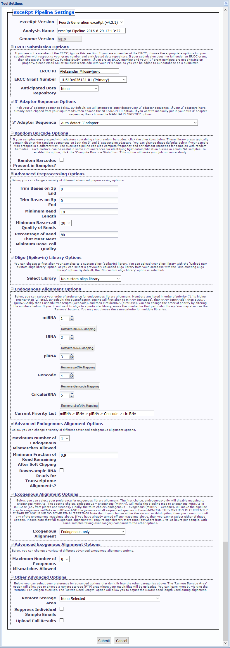
exceRpt has many different options (see our tutorial for more information!), but we're only going to change three of them for this submission.
First, we will update the Analysis Name so that it includes some additional information about our submission.
The analysis name will be used to organize the output files from your submission.
We recommend that you always keep a timestamp of some kind in your analysis name, as it'll help you remember when you submitted each analysis.

Second, we will update 3' Adapter Sequence from "Auto-detect 3' adapter" to "MANUALLY SPECIFY 3' ADAPTER".
Then, in the Manual Input of 3' Adapter Sequence option that appears, we will put AGATCGGAAGAGCACACGTCT.
We are providing the 3' adapter sequence manually (as opposed to having exceRpt guess the sequence) because these samples have a 3' adapter sequence which is not in exceRpt's standard adapter sequence library.

Third, we will enable the Suppress Individual Sample Emails option. Normally, you will receive one email for each sample that is processed - since we are submitting 40 samples, we don't want to receive 40 emails!
This option will suppress these individual sample emails, but you will still receive a few other emails informing you about the progress of your submission.
The option can be found under the Other Advanced Options menu at the bottom of the tool dialog - you will need to expand the menu by clicking the *+*.

After changing these three settings, we'll click Submit.
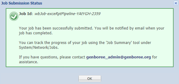
You should see a notification informing you that your samples have been submitted:

Before proceeding to part 3 of the tutorial, you'll need to wait for your samples to be processed.
Depending on how busy our cluster is, this could take several hours.
If you don't want to wait, you can access the same results via the Examples and Test Data group:

Tutorial, Part 3: Performing Deconvolution¶

• An archive containing RPM-normalized read counts (created by exceRpt)
• A text file providing metadata about the samples

We'll describe how to find and/or create both files below.

1) Finding Your exceRpt Results and Input Data File¶

After your samples have been processed, you'll want to find the results created by exceRpt.
You'll find those results in your database organized by the analysis name you provided:

If you're interested in learning more about your results, you can read our data analysis tutorial.
However, for the deconvolution tool, we're really only interested in one file:

This archive contains RPM-normalized read counts for all of the different ncRNA species mapped by exceRpt (miRNA / piRNA / tRNA / GENCODE annotations / circular RNA).
These read counts are the input data for the deconvolution tool.
Your file will have a slightly different name than mine because your analysis name is different.

2) Creating Your Metadata Text File¶

The second file required by the deconvolution tool is a text file that contains metadata describing the samples.
You can find an example of this metadata text file in the Examples and Test Data group:

• Each row contains a sample name
• Each column contains a metadata attribute ("biofluid" and "condition", in this case).
• Each sample is labeled by biofluid ("Plasma" or "Urine") and by condition ("Healthy Control").

When you're working with your own samples, you'll create your own metadata file describing your samples and upload it to your database.

IMPORTANTLY, the sample names provided in your metadata file must match the output generated by exceRpt.
During processing, exceRpt will transform the names of your FASTQ files by inserting "sample_" at the beginning and substituting underscores ("_") for any periods, pipes ("|"), or spaces.
To verify that you are providing the correct sample names in your metadata file, you can download the _exceRpt_miRNA_ReadsPerMillion.txt file generated by exceRpt and double-check that the sample names in your metadata file match what is provided there:

For the tutorial, you can just drag our pre-made file into the Input Data panel.
Finally, make sure that you dragged your database to the Output Targets panel.
Your Workbench should now look something like this:

3) Running the Deconvolution Tool¶

To run the deconvolution tool, select exRNA Computational Deconvolution from the tool menu at the top of the Workbench:

This tool is much simpler than exceRpt - just provide an updated analysis name (much like you did when launching your exceRpt analysis) and click the Submit button.
The tool will likely only take a few minutes to run. Upon completion, you will receive an email informing you that your analysis is ready.

4) Downloading Your Deconvolution Results¶

Your deconvolution results will be uploaded to your database organized by the analysis name you provided:

You can select any of the output files (explained in more detail below) and then click the "Click to Download File" link in the Details panel to download the output file.
In particular, we recommend downloading the _deconvolutionResults archive, as it will contain all results generated by the tool.

5) Understanding Your Deconvolution Results¶

Output from the tool includes:

• Stage 1 Deconvolution Results
  • Stage 1_Results_Boxplots.pdf - Boxplots of the per-sample proportions for each estimated constituent cargo profile (rows) numbered 1 through k. Boxplots are separated based on metadata columns (e.g., disease, biofluid, etc.).
  • Stage1_Results_Expression.txt - exRNA expression in transformed transcript abundance values (rows) for each estimated constituent cargo profile (columns) numbered 1 through k (profiles modeled for the input dataset).
  • Stage1_Results_Heatmap_Correlations.pdf - Estimated constituent cargo profiles (rows) are correlated using the exRNA expression in transformed transcript abundance values across the informative RNAs (see Murillo et al., 2019) against the 6 CTs (columns) previously identified through the deconvolution of the exRNA Atlas (see Murillo et al., 2019).
  • Stage1_Results_Heatmap_Proportions.pdf - Heatmap of the per-sample proportions (columns) for each estimated constituent cargo profile (rows) numbered 1 through k. Dendrogram is included to cluster similar composed samples.
  • Stage1_Results_Proportions.txt - Per-sample proportions (columns) for each estimated constituent cargo profile (rows) numbered 1 through k (profiles modeled for the input dataset).
• Stage 2 Deconvolution Results
  • NOTE: Stage 2 deconvolution is performed for each metadata value that is associated with at least 20 samples.
  • Stage2_[METADATA COLUMN]_[METADATA VALUE]_miRNA_RPM.txt - Tables of estimated average cargo profiles across miRNA transcripts in reads per million (rows) separated based on provided metadata values. Columns include mean expression and std. errors for each estimated constituent cargo profile (numbered 1 through k) as well as degrees of freedom, explained variances, and per sample residuals.

You can ignore the jobFile.json file. This file just contains various internal settings used to process your submission.

Troubleshooting¶

• Make sure that the row headers in the sample descriptor file match the sample names generated by exceRpt.
  • The sample names generated by exceRpt are based on the file names of the inputs used for exceRpt.
  • Remember that you can see the relevant list of sample names by viewing the exceRpt_miRNA_ReadsPerMillion.txt file (located in the postProcessedResults_v4.6.3 directory).
• Make sure that your submission contains data from at least 40 samples. Submissions with lower numbers of samples will fail processing (as the tool's underlying algorithm requires at least 40 samples to work properly).
• For Stage 2, metadata values must be associated with at least 20 samples in order to be processed. Any metadata values associated with fewer than 20 samples will be skipped during this stage of the tool.

References and Attributions¶

1. Onuchic, V., Hartmaier, R.J., Boone, D.N., Samuels, M.L., Patel, R.Y., White, W.M., Garovic, V.D., Oesterreich, S., Roth, M.E., Lee, A.V., et al. (2016). Epigenomic Deconvolution of Breast Tumors Reveals Metabolic Coupling between Constituent Cell Types. Cell Reports 17, 2075–2086.
2. Tool designed and implemented by Oscar D. Murillo at the Bioinformatics Research Lab, Baylor College of Medicine, Houston, TX.
3. Integrated into the Genboree Workbench by William Thistlethwaite at the Bioinformatics Research Lab, Baylor College of Medicine, Houston, TX.

• Fold Change Calculation Using DESeq2
• Introduction
• Preliminary Steps for Setting Up Any Analysis in the Genboree Workbench
• Create a Group for Your Analysis
• Create a Database for Your Analysis
• Upload your Data File(s)
• Step-by-step Instructions to Set Up Job
• Example Data for Running DESeq2
• Output Files Generated by Job
• References and Attributions

Fold Change Calculation Using DESeq2¶

Introduction¶

This tool will test samples for differential expression using DESeq2 (version 1.6.3).
Currently, the tool allows you to test a given factor (disease, for example) across two different factor levels (control versus Alzheimer's disease, for example).
We will continue to develop this tool and will add new features (like allowing analysis over multiple factors) in the coming months.

Preliminary Steps for Setting Up Any Analysis in the Genboree Workbench¶

Create a Group for Your Analysis¶

FAQ

What is a Group?

A "Group" contains Databases and Projects and controls access to all content within. You control access to your Group(s), and who is a member of your group. You can also belong to multiple Groups (i.e. collaborators).

This step is optional. You can also use your default/existing group.

Create a Database for Your Analysis¶

FAQ

What is a Database?

A "Database" contains Tracks, Lists, Sample Sets, Samples, and Files. Each database can be associated with a reference genome.

This step is required.
Make sure that you pick the proper reference sequence genome (hg19, for example) when creating your database.
Note that we do not have an entry for hg38 or mm10 in our "Reference Sequence" list.
If your data is associated with either of these reference sequence genomes, follow the directions below.

Create a Database for hg38 or mm10

In order to create a database associated with hg38 or mm10, select the "User Will Upload" option for "Reference Sequence"
and provide appropriate values for the Species and Version text boxes as given below:

If your genome of interest is not available, please contact the exRNA Team for help.

Upload your Data File(s)¶

FAQ

What types of files can be uploaded?

The Fold Change Calculating Using DESeq2 tool accepts exactly two text files as input.
One file should contain your miRNA read counts, with rows corresponding to miRNA identifiers and columns corresponding to individual sample names.
The other file should contain your sample descriptors, with rows corresponding to individual sample names and columns corresponding to factor names ("condition", "biofluid", etc.).

Step-by-step Instructions to Set Up Job¶

1. Drag exactly two text files (with the formatting described above) into the Input Data panel. You can also drag a folder or file entity list if it contains both text files.
2. Drag a Database to the Output Targets panel to store results.
3. Select Transcriptome » Differential Expression Analysis » Fold Change Calculating Using DESeq2 from the Toolset menu.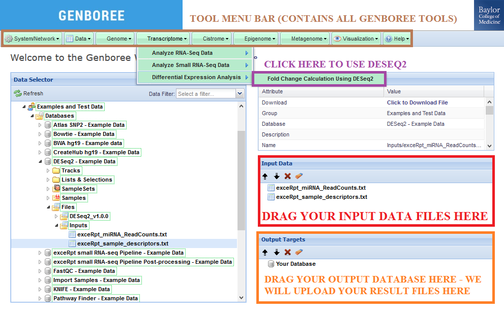
   
4. Fill in the analysis name for your tool job. We recommend keeping a timestamp in your analysis name!
5. Fill in the factor name and the corresponding factor levels for your analysis. For example, if I was using the tutorial files and wanted to examine the "disease" factor and compare "AD" (Alzheimer's disease) to "CONTROL" (healthy controls), I would put the following values:
   • Factor Name: disease
   • Factor Level 1: AD
   • Factor Level 2: CONTROL
6. Select the different ERCC-related submission settings if you are a member of the ERCC. If you are not, then ignore this section.
7. Choose to upload your results to a remote storage area if you wish to do so. More information about this option can be found here.
8. Submit your job. Upon completion of your job, you will receive an email.
9. Download the results of your analysis from your Database. The results data will end up under the DESeq_v1.0.0 folder in the Files area of your output database.
   • Within that folder, your Analysis Name will be used as a sub-folder to hold the files generated by that run of the tool.
   • Open this sub-folder to see your results.
   • Select any of the output files (explained in more detail below) and then click the link Click to Download File from the Details panel to download that output file.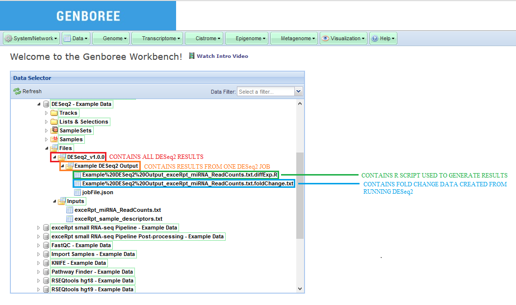
     

Example Data for Running DESeq2¶

In this example, we have used a set of miRNA read counts processed by exceRpt for 181 different samples (found in exceRpt_miRNA_ReadCounts.txt).
We have also used a sample descriptor document which contains information about disease and biofluid for each of the 181 samples (found in exceRpt_sample_descriptors.txt).

The sample input files and output results can be found here:

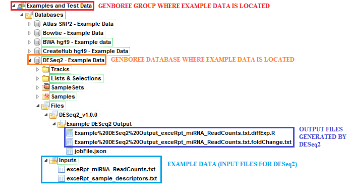
• Under the group Examples and Test Data, select the database DESeq2 - Example Data.
• Both input files can be found in the folder: Files » Inputs.
• DESeq2 results can be found under the Files » DESeq2_v1.0.0 » Example DESeq2 Output folder in this database.

Output Files Generated by Job¶

After your job successfully completes, you will be able to download 2 different output files:

• A _foldChange.txt file that contains the results from your DESeq2 analysis.
• A _diffExp.R file that is the R script used to generate your results.

References and Attributions¶

1. M. I. Love, W. Huber, S. Anders: Moderated estimation of fold change and dispersion for RNA-seq data with DESeq2. Genome Biology 2014, 15:550. http://dx.doi.org/10.1186/s13059-014-0550-8
2. Integrated into the Genboree Workbench by William Thistlethwaite and Sai Lakshmi Subramanian at the Bioinformatics Research Laboratory, Baylor College of Medicine, Houston, TX.

This tool has been deployed in the context of the exRNA Communication Consortium (ERCC).
Please contact the exRNA Team with questions or comments, or for help using it on your own data.

• ExRNA Data Analysis Using the exceRpt small RNA-seq Pipeline
• Step 1: Look at Your .stats File
• Step 2: Look at the Contents of your CORE_RESULTS Archive
• Step 3 (Optional): Look at the Contents of Your Full Results Archive
• Step 4 (Optional): Look at Post-processed Results

ExRNA Data Analysis Using the exceRpt small RNA-seq Pipeline¶

Much of the material on this page has been taken from the exceRpt GitHub page.
Many of the files generated by exceRpt for a given sample will include that sample's name.
We use the term [sampleName] to refer to this name in a general sense.

Step 1: Look at Your .stats File¶

The first place to look when trying to understand your results is the .stats file.
Your .stats file can be found directly inside the directory associated with your exceRpt run on Genboree.
It can also be found in the CORE_RESULTS archive generated from your exceRpt run (further described below).
This file summarizes the number of reads that map to each class of targets in the pipeline.
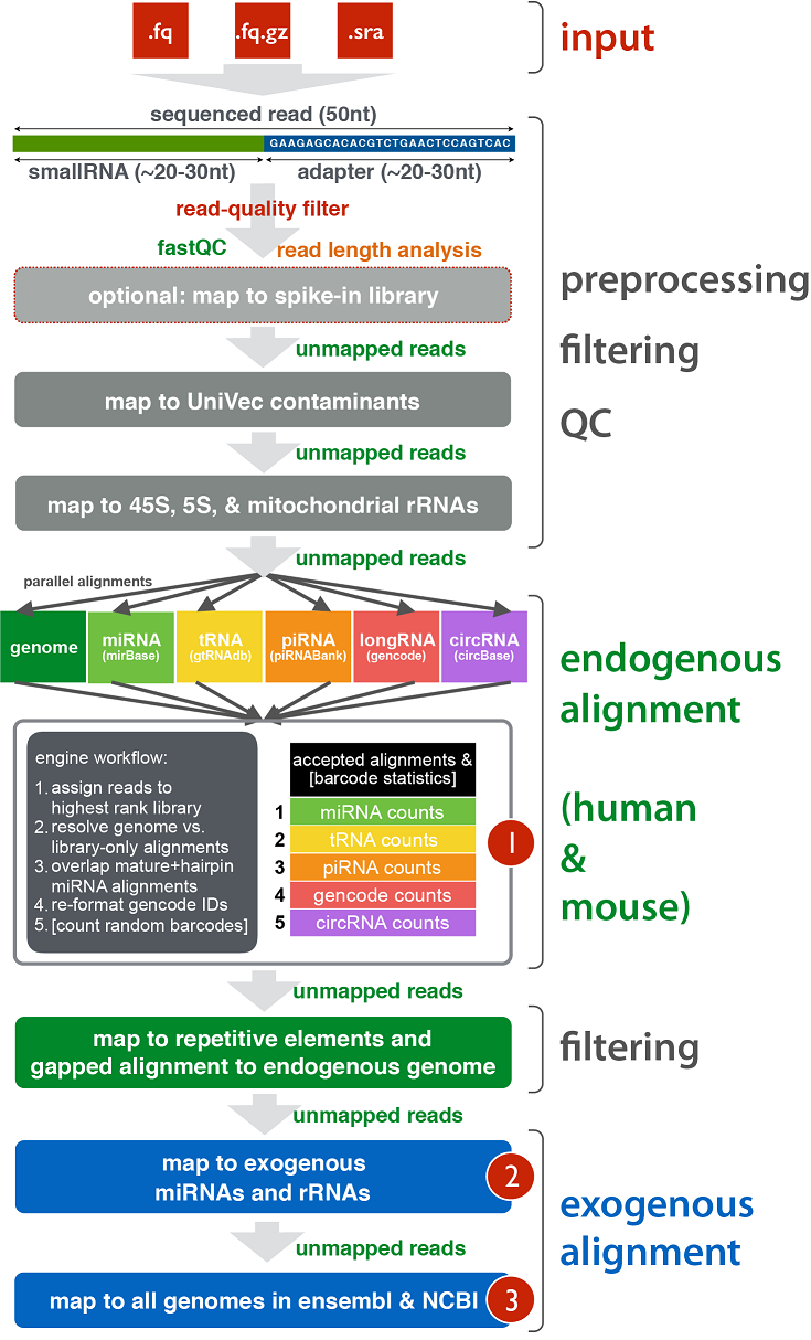
In order to better understand how the pipeline maps to each class of targets (endogenous miRNAs, tRNAs, exogenous miRNAs, etc.), click here.
This link contains a useful infographic and an explanation of how the pipeline works.

Here is an example output for a .stats file:

#STATS from the exceRpt smallRNA-seq pipeline v.4.3.2 for sample sample_C5_non_pregnant5_SRR822437_fastq. Run started at 2016-07-12--12:03:16
Stage    ReadCount
input    1291553
successfully_clipped    1291498
failed_quality_filter    138130
failed_homopolymer_filter    49
calibrator    NA
UniVec_contaminants    32636
rRNA    23020
reads_used_for_alignment    1097663
genome    72996
miRNA_sense    26683
miRNA_antisense    0
miRNAprecursor_sense    386
miRNAprecursor_antisense    1
tRNA_sense    1685
tRNA_antisense    0
piRNA_sense    0
piRNA_antisense    0
gencode_sense    7189
gencode_antisense    3555
circularRNA_sense    0
circularRNA_antisense    0
not_mapped_to_genome_or_libs    1024667
#END OF STATS from the exceRpt smallRNA-seq pipeline. Run completed at 2016-07-12--15:15:46

The .stats file above was generated by an exceRpt run with exogenous mapping disabled (endogenous-only).
Your .stats file will have more information if you choose a different exogenous mapping setting.
If you choose the "endogenous + exogenous (miRNA)" setting, your .stats file will have the following extra lines:

repetitiveElements    2080
endogenous_gapped    11627
input_to_exogenous_miRNA    1010951
exogenous_miRNA    9
input_to_exogenous_rRNA    1010942
exogenous_rRNA    852

Finally, if you choose the most extensive exogenous option, "endogenous + exogenous (miRNA + Genome)", your .stats file will also have these lines:

input_to_exogenous_genomes    1010090
exogenous_genomes 2807

You can learn more about the different exogenous settings by viewing the tutorial on exceRpt's settings.

Step 2: Look at the Contents of your CORE_RESULTS Archive¶

The next place to look for your analysis is the CORE_RESULTS archive uploaded with every successful exceRpt run.
This archive will be sufficient for most analyses.
We decompress the archive for you in the Genboree Workbench - you can find its contents in the CORE_RESULTS sub-folder associated with a particular run.

When you decompress your CORE_RESULTS archive (or look at the contents on Genboree), you will immediately see the following files in the base directory:

In general, you shouldn't need to look at the .log file. It contains a detailed log of the different steps performed during the course of the pipeline.
We are happy to look at the .log file to help you if something goes wrong with exceRpt or if you have a question for us.
The .qcResult file will contain data for the QC metrics discussed here.
In addition, the transcriptome complexity provided in the .qcResult file is calculated by dividing the total number of unique sequence alignments by the total number of sequence alignments when aligning to the transcriptome.
The alignments used in this calculation are taken from the endogenousAlignments_Accepted.txt.gz file (described in more detail below and only available in the full results archive).

The .stats file was discussed above.

There will be a folder in your CORE_RESULTS archive that matches the name of your sample. That folder will contain the following files:

If you chose the "endogenous + exogenous (miRNA)" setting (mapping to exogenous miRNA / rRNA),
there will be an additional subfolder named EXOGENOUS_miRNA which will include some additional readCounts files
for exogenous miRNA. There are no readCounts files for exogenous rRNA.

Finally, if you chose the "endogenous + exogenous (miRNA + Genome)" setting (mapping to all of the above as well as exogenous genomes),
there will be an additional subfolder named EXOGENOUS_genomes which will include a taxonomy tree file
named ExogenousGenomicAlignments.result.taxaAnnotated.txt.
This text file will provide taxonomy information about the different taxons found in your sample.

When looking at the files above, you'll probably be most interested in the readCounts files.
An example of how these files are formatted can be seen below:

Below, you can see a description of each column:

• ReferenceID is the ID of each annotated RNA.
• uniqueReadCount is the number of unique insert sequences attributed to each annotated RNA.
• totalReadCount is the total number of reads attributable to each annotated RNA.
• multimapAdjustedReadCount is the count after adjusting for multi-mapped reads.
• multimapAdjustedBarcodeCount (available only for samples prepped with randomly barcoded 5' and/or 3' adapters such as Bioo) is the number of unique N-mer barcodes
  adjusted for multimapping ambiguity in the insert sequence.

If your exceRpt run didn't map to a given library, there will be no corresponding readCounts file in your CORE_RESULTS archive.
For example, if you didn't have any tRNA sense reads, there will be no [sampleName].readCounts_tRNA_sense.txt file.

Step 3 (Optional): Look at the Contents of Your Full Results Archive¶

If the files given above are not sufficient, you can select the "Upload Full Results" option when launching your exceRpt job.
This will make your exceRpt job upload an archive containing all files created by exceRpt during the processing of your sample(s).
This means that your full results archive will contain all of the files located in your CORE_RESULTS archive.
Because some of the files inside this archive can be large, it is not recommended to choose this option unless you absolutely need these files.

When you open this archive, you will see a folder with your sample name (just like the CORE_RESULTS archive).
Inside that folder, you will see the following types of files:

Intermediate files containing reads 'surviving' each stage

1. 3' adapter clipping
2. 5'/3' end trimming
3. read-quality and homopolymer filtering
4. UniVec contaminant removal
5. rRNA removal
6. Transcriptome alignments (ungapped) of reads mapped to the genome
7. Transcriptome alignments (ungapped) of reads not mapped to the genome
8. Repetitive elements (only present if exogenous mapping is being done)
9. Genome allowing gaps / novel splices (only present if exogenous mapping is being done)
10. Exogenous miRNA (only present if exogenous mapping is being done)
11. Exogenous rRNA (only present if exogenous mapping is being done)

The names of these files will look like the following:

The one exception is the read file associated with reads remaining after exogenous rRNA alignment.
This file ends in .fq.gz.

Reads aligned at each step of the pipeline

1. UniVec
2. rRNA
3. endogenous genome
4. endogenous transcriptome

The names of these files will look like the following:

Alignment summary information obtained after invoking the library priority

By default, the library priority will choose a miRBase alignment over any other alignment.
For example, if a read is aligned to both a miRNA in miRBase and a miRNA in Gencode, the miRBase alignment is kept and all others discarded.
It is especially important for tRNAs to be chosen in favour of piRNAs, as the latter have quite a large number of misannotations compared to the former.

The names of these files will look like the following:

Step 4 (Optional): Look at Post-processed Results¶

If you submitted dozens or even hundreds of samples for processing, you might not want to crawl through each sample's read count files.
In this situation, we recommend looking at your submission's post-processed results.
This tool combines the information from each sample into comprehensive files that cover all of the samples.
For example, if you submitted 100 samples for processing, you could look at the [analysisName]_miRNA_ReadCounts.txt file
in your post-processed results to see miRNA read counts for all 100 samples at the same time.

You can learn more about these results here.

• Detecting Circular and Linear Isoforms from RNA-seq Data Using KNIFE
• Introduction
• Preliminary Steps for Setting Up Any Analysis in the Genboree Workbench
• Create a Group for Your Analysis
• Create a Database for Your Analysis
• Upload your Data File(s)
• Step-by-step Instructions to Set Up KNIFE Submission
• Notes for Preparing Input Data Files
• Example Data for Running KNIFE
• Summary of Output Files Generated by KNIFE
• Detailed Explanation of Output Files Generated by KNIFE
• References and Attributions

Detecting Circular and Linear Isoforms from RNA-seq Data Using KNIFE¶

Introduction¶

This tool performs statistically based splicing detection for circular and linear isoforms from RNA-Seq data.
The tool's statistical algorithm increases the sensitivity and specificity of circularRNA detection from RNA-Seq data by quantifying circular and linear RNA splicing events at both annotated and un-annotated exon boundaries.

Preliminary Steps for Setting Up Any Analysis in the Genboree Workbench¶

Create a Group for Your Analysis¶

FAQ

What is a Group?

A "Group" contains Databases and Projects and controls access to all content within. You control access to your Group(s), and who is a member of your group. You can also belong to multiple Groups (i.e. collaborators).

This step is optional. You can also use your default/existing group.

Create a Database for Your Analysis¶

FAQ

What is a Database?

A "Database" contains Tracks, Lists, Sample Sets, Samples, and Files. Each database can be associated with a reference genome.

This step is required.
Make sure that you pick the proper reference sequence genome (hg19, for example) when creating your database.

The KNIFE tool currently supports the following genomes: hg19, mm10, rn5, and dm3.
However, we do not have entries for mm10, rn5, or dm3 in the reference sequence list within our Create Database tool.

If you want to create a Database associated with mm10, rn5, or dm3, select the "User Will Upload" option for "Reference Sequence".
Then, provide appropriate values for the Species and Version text boxes, as given below:

All data (inputs and outputs) associated with a given genome should go into that Database.
For example, if you create an hg19 Database, then all of your hg19 data belongs in that Database.
If you have other data that corresponds to another reference genome (mm10, for example), then you should create a second Database to hold that data.

Upload your Data File(s)¶

FAQ

What types of files can be uploaded?

• Examples: SAMPLENAME_1.fastq and SAMPLENAME_2.fastq, SAMPLENAME_R1.fq and SAMPLENAME_R2.fq

Your inputs can be compressed in one large archive, multiple archives, etc.
All that matters for processing is that your paired-end FASTQ file names (not the archives containing the FASTQ files!) must follow the naming convention above.
Single-end files should either NOT include a suffix or should end in _1 or _R1.

Step-by-step Instructions to Set Up KNIFE Submission¶

1. Drag one or more FASTQ files to the Input Data panel. The input file(s) can be compressed.
   Optionally, you can also upload one or more compressed archives of multiple FASTQ files. Each FASTQ file can also be compressed inside these archives.
   Then, you can drag these multiple input file archives to the Input Data panel.
   Check out the Notes below for more info on preparing your input data files.
2. Drag a Database to the Output Targets panel to store results.
3. Select Transcriptome » Analyze Small RNA-Seq Data » exRNA Data Analysis » KNIFE (Known and Novel IsoForm Explorer) from the Toolset menu.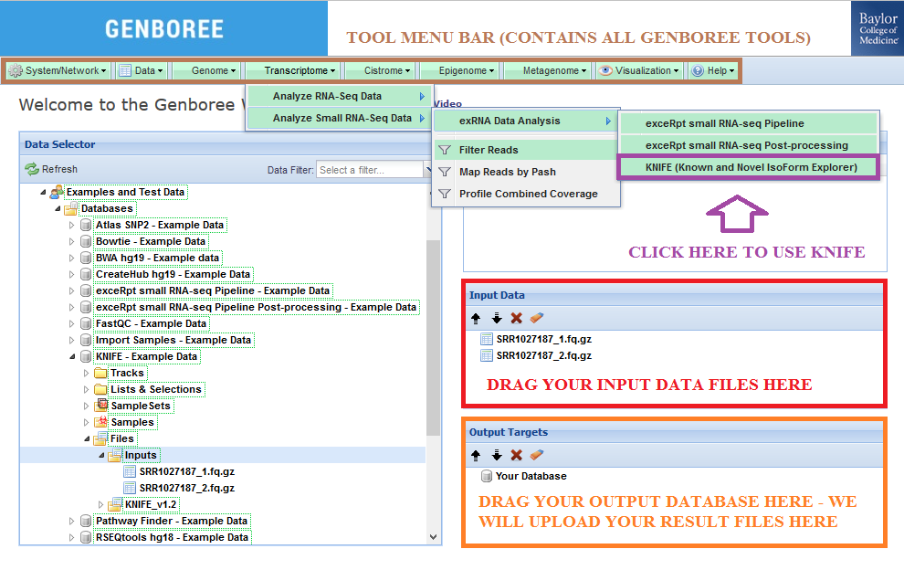
   
4. Fill in the analysis name for your tool job. We recommend keeping a timestamp in your analysis name!
5. Select the different ERCC-related submission settings if you are a member of the ERCC. If you are not, then ignore this section.
6. Choose to upload your results to a remote storage area if you wish to do so. More information about this option can be found here.
7. Submit your job. Upon completion of your job, you will receive an email.
8. Download the results of your analysis from your Database. The results data will end up under the KNIFE_v1.2 folder in the Files area of your output database.
   • Within that folder, your Analysis Name will be used as a sub-folder to hold the files generated by that run of the tool.
   • Open this sub-folder to see your results.
   • Select any of the output files (explained in more detail below) and then click the link Click to Download File from the Details panel to download that output file.

Notes for Preparing Input Data Files¶

RECOMMENDATION:

• If you have a large number of input FASTQ files, it is highly recommended to make smaller archives with fewer number of input files
  in order to avoid issues with uploading them to your Genboree Database.
  • Each compressed archive should not be larger than 10GB.
  • Upload all of your smaller archives to your Genboree Database and then submit them all in the same KNIFE job.
  • This technique will allow you to successfully upload many input files and compare/contrast results from those input files in one job submission.

IMPORTANT NOTES:

• If you are using Mac OS to prepare your files, remember to remove the "__MACOSX" sub-directory that gets added to the compressed archives.
• In order to create your archive using the terminal, first navigate to the directory where your files are.
  • EXAMPLE: If my files were located in C:/Users/John/Desktop/Submission, I would use the "cd" command in my terminal and type
    

    cd C:/Users/John/Desktop/Submission
    

  • Next, you will use the zip command with the -X parameter (to avoid saving extra file attributes) to compress your files.
  • EXAMPLE: Imagine that I am submitting 4 data files : inputSequence1.fq.gz, inputSequence2.fq.bz2, inputSequence3.fq.zip, inputSequence4.sra
    I want to name my .zip file johnSubmission.zip
    • I would type the following:
      

      zip -X johnSubmission.zip inputSequence1.fq.gz inputSequence2.fq.bz2 inputSequence3.fq.zip inputSequence4.sra
      

• Commonly used compression formats like .zip, .gz, .tar.gz, .bz2 are accepted.

Example Data for Running KNIFE¶

In this example, we have used a single sample with paired end read data from a human sample. Raw reads were grabbed from SRA, and
TrimGalore (wrapper for cutadapt) was used to trim poor quality ends and the adapter sequence. The original reads were 60nt - after
trimming, we kept all reads where both mates were at least 50nt. The FASTQ files use phred64 encoding (which is required).

The sample input FASTQ files and output results can be found here:

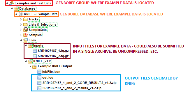
• Under the group Examples and Test Data, select the database KNIFE - Example Data.
• Both compressed input files can be found in the folder: Files » Inputs.
• KNIFE results can be found under the Files » KNIFE_v1.2 » Example KNIFE Output folder in this database.
  • In particular, the SRR1027187_1_and_2 subfolder contains the result files generated for the SRR1027187_1 and SRR1027187_2 paired end reads.
  • Each processed sample is given its own dedicated folder.

Summary of Output Files Generated by KNIFE¶

After your job successfully completes, you will be able to download 3 different output files:

• A _results_v1.2.zip file that contains all of the result files from your KNIFE run.
  • This file will be quite large (gigabytes) because it includes all of the full alignment files for your run.
• A _CORE_RESULTS_v1.2.zip file that contains all of the result files from your KNIFE run, minus the full alignment files.
  • This file is a good alternative to the full results archive, as it is significantly smaller (the archive will be ~150 megabytes).
• An out.log file that contains output generated by the KNIFE run.

Detailed Explanation of Output Files Generated by KNIFE¶

Within the full results archive, you will find four different subdirectories located in /outputs/[sample name]. These subdirectories are detailed in full below:

1. circReads: The primary output files you will be interested in looking at are in the following subdirectories.
   • reports: read count and p-value per junction using naive method. 2 files created per sample, 1 for annotated junctions (linear and circular) and the other for de novo junctions.
     For single end reads and de novo junctions from either single end or paired end data, these are the output files of interest as GLM reports are for annotated junctions using paired end data only.
     You will want to select a threshold on the p-value for which of these junctions are considered true positive circles.
     For the publication, we considered all junctions with a p-value of 0.9 or higher and a decoy/circ read count ratio of 0.1 or lower.
     • junction: chr|gene1_symbol:splice_position|gene2_symbol:splice_position|junction_type|strand
       • junction types are reg (linear), rev (circle formed from 2 or more exons), or dup (circle formed from single exon)
     • linear: number of reads where read1 aligned to this linear junction and read2 was consistent with presumed splice event, or just number of aligned reads to this linear junction for SE reads
     • anomaly: number of reads where read2 was inconsistent with read1 alignment to this linear junction
     • unmapped: number of reads where read1 aligned to this junction and read2 did not map to any index
     • circ: number of reads where read1 aligned to this circular junction and read2 was consistent with presumed splice event, or just number of aligned reads to this circular junction for SE reads
     • decoy: number of reads where read2 was inconsistent with read1 alignment to this circular junction
     • pvalue: naive method p-value for this junction based on all aligned reads (higher = more likely true positive).
       You will want to select a threshold on the p-value for which of these junctions are considered true positive circles.
     • scores: (read1, read2) Bowtie2 alignment scores for each read aligning to this junction, or scores at each 10th percentile for junctions with more than 10 reads
   • glmReports: read count and posterior probability per junction using GLM (only for PE reads, annotation-dependent junctions).
     2 files created per sample, 1 with circular splice junctions and the other with linear splice junctions.
     You will want to select a threshold on the posterior probability for which of these junctions are considered true positive circles.
     For the publication, we considered all junctions with a posterior probability of 0.9 or higher.
     • junction: chr|gene1_symbol:splice_position|gene2_symbol:splice_position|junction_type|strand
       • junction types are reg (linear), rev (circle formed from 2 or more exons), or dup (circle formed from single exon)
     • numReads: number of reads where read1 aligned to this junction and read2 was consistent with presumed splice event
     • p_predicted: posterior probability that the junction is a true junction (higher = more likely true positive).
     • p_value: p-value for the posterior probability to control for the effect of total junctional counts on posterior probability
   • glmModels: RData files containing the model used to generate the glmReports
   • ids: alignment and category assignment per read
2. sampleStats: Contains 2 txt files with high-level alignment statistics per sample (read1 and read2 reported separately).
   • SampleAlignStats.txt: useful for evaluating how well the library prep worked, for example ribosomal depletion.
     Number of reads are reported, with fraction of total reads listed in ()
     • READS: number of reads in original fastq file
     • UNMAPPED: number of reads that did not align to any of the junction, genome, transcriptome, or ribosomal indices
     • GENOME: number of reads aligning to the genome
     • G_STRAND: percentage of GENOME reads aligning to forward strand and percentage aligning to reverse strand
     • TRANSCRIPTOME: number of reads aligning to the transcriptome
     • T_STRAND: percentage of TRANSCRIPTOME reads aligning to forward strand and percentage aligning to reverse strand
     • JUNC: number of reads aligning to the scrambled or linear junction index and overlapping the junction by required amount
     • J_STRAND: percentage of JUNC reads aligning to forward strand and percentage aligning to reverse strand
     • RIBO: number of reads aligning to the ribosomal index
     • R_STRAND: percentage of RIBO reads aligning to forward strand and percentage aligning to reverse strand
     • 28S, 18S, 5.8S, 5SDNA, 5SrRNA: percentage of RIBO aligning to each of these ribosomal subunits (for human samples only)
     • HBB: number of reads aligning to HBB genomic location (per hg19 annotation)
   • SampleCircStats.txt: useful for comparing circular and linear ratios per sample
     • CIRC_STRONG: number of reads that aligned to a circular junction that has a p-value >= 0.9 using the naive method (very high confidence of true circle)
     • CIRC_ARTIFACT: number of reads that aligned to a circular junction that has a p-value < 0.9 using the naive method
     • DECOY: number of reads where read2 did not align within the circle defined by read1 alignment
     • LINEAR_STRONG: number of reads that aligned to a linear junction that has a p-value >= 0.9 using the naive method (very high confidence of true linear splicing)
     • LINEAR_ARTIFACT: number of reads that aligned to a linear junction that has a p-value < 0.9 using the naive method
     • ANOMALY: number of reads where read2 did not support a linear transcript that includes the read1 junction alignment
     • UNMAPPED: number of reads where read1 aligned to a linear or scrambled junction but read2 did not map to any index
     • TOTAL: sum of all previous columns, represents total number of reads mapped to junction but not to genome or ribosome
     • CIRC_FRACTION: CIRC_STRONG / TOTAL
     • LINEAR_FRACTION: LINEAR_STRONG / TOTAL
     • CIRC / LINEAR: CIRC_FRACTION / LINEAR_FRACTION
3. orig: contains all sam/bam file output and information used to assign reads to categories.
   In general there is no reason to dig into these files since the results, including the ids of reads that aligned to each junction, are output in report files under circReads as described above,
   but sometimes it is useful to dig back through if you want to trace what happened to a particular read.
   • genome: sam/bam files containing Bowtie2 alignments to the genome index
   • junction: sam/bam files containing Bowtie2 alignments to the scrambled junction index
   • reg: sam/bam files containing Bowtie2 alignments to the linear junction index
   • ribo: sam/bam files containing Bowtie2 alignments to the ribosomal index
   • transcriptome: sam/bam files containing Bowtie2 alignments to the transcriptome index
   • unaligned: fastq and fasta files for all reads that did not align to any index
     • forDenovoIndex: fastq files containing subset of the unaligned reads that are long enough to be used for creating the denovo junction index
   • denovo: sam/bam files containing Bowtie2 alignments to the de novo junction index
   • still_unaligned: fastq files containing the subset of the unaligned reads that did not align to the denovo index either
   • ids: text files containing the ids of reads that aligned to each index, location of alignment, and any other relevant data from the sam/bam files used in subsequent analysis.
     The reads reported in the junction and reg subdirectories are only those that overlapped the junction by user-specified amount.
     In juncNonGR and denovoNonGR, the reported read ids are the subset of reads that overlapped a junction and did not align to the genome or ribosomal index.
4. denovo_script_out: debugging output generated during creation of de novo index.

The core results archive will contain all of the files above except for the orig directory (which contains all sam/bam file output and is very large).

References and Attributions¶

1. Szabo L, Morey R, Palpant NJ, Wang PL, Afari N, Jiang C, Parast MM, Murry CE, Laurent LC, Salzman J. Statistically based splicing detection reveals neural enrichment and tissue-specific induction of circular RNA during human fetal development. Genome Biology. 2015, 16:126. http://www.ncbi.nlm.nih.gov/pubmed/26076956
2. Integrated into the Genboree Workbench by William Thistlethwaite and Sai Lakshmi Subramanian at the Bioinformatics Research Laboratory, Baylor College of Medicine, Houston, TX.

This tool has been deployed in the context of the exRNA Communication Consortium (ERCC).
Please contact Emily LaPlante with questions or comments, or for help using it on your own data.

• Long RNA-Seq Data Analysis Using RSEQtools in the Genboree Workbench
• Preliminary Steps to Set Up Any Analysis in the Genboree Workbench
• Step-by-step Instructions to Set Up Long RNA-Seq Data Analysis
• Example Data for Running RSEQtools
• RSEQTools Pipeline - Workflow Implemented in the Genboree Workbench
• RSEQtools Modules used in Genboree Implementation
• References and Attributions

Long RNA-Seq Data Analysis Using RSEQtools in the Genboree Workbench¶

View Screencast (no audio)

Preliminary Steps to Set Up Any Analysis in the Genboree Workbench¶

• Create a Group for your analysis - FAQ. This step is optional. You can also use your default/existing group.

  What is a Group?

  A "Group" contains Databases and Projects and controls access to all content within. You control access to your Group(s), and who is a member of your group. You can also belong to multiple Groups (i.e. collaborators).

• Create a Database for your analysis - FAQ. This step is optional. You can also use your default/existing database.

  What is a Database?

  A Database contains Tracks, Lists, Sample Sets, Samples, and Files. Each database can be associated with a reference genome.

• Create a Redmine Project for your analysis - FAQ. This step is REQUIRED.

  What is a Redmine Project?

  The Redmine Project holds files (HTML, plots, etc) that contain analysis results from your tool.

• Upload your data file(s) - FAQ

  What type of files can be uploaded?

  The long RNA-Seq pipeline using RSEQtools accepts a single-end or paired-end FASTQ files as input. The input files can be compressed.

Step-by-step Instructions to Set Up Long RNA-Seq Data Analysis¶

1. Drag Single or paired-end FASTQ files to Input Data panel. The input files can be compressed.
2. Drag a Database and a Project to Output Targets panel to store results.
3. Select Transcriptome » Analyze RNA-Seq Data » Analyze RNA-Seq data by RSEQtools from the Toolset menu.
4. Fill in appropriate details in the Tool Settings dialog box
5. Submit your job. Upon completion of your job, you will receive an email.
6. Download the results of your analysis from your Database. The results data will end up under the RSEQtools folder in the Files area of your output database.
   Within that folder, your Analysis Name will be used as a sub-folder to hold the files generated by that run of the tool.
   • Click on your results file(s) in the Data Selector panel.
   • Select the link Click to Download File from the Details panel to download your results file(s).
7. View plots from the Projects page.
   • Click on your project name in the Data Selector panel.
   • Click on Link to Project in the Details panel to view your Projects page.
8. If you would like to visualize your signal tracks in the UCSC Genome Browser, follow these steps:
   • Drag your Database to Output Targets panel.
   • Select Data » Databases » Unlock/Lock Database from the Toolset menu.
   • Click Submit in the Setting Dialog box to unlock your database.
   • Clean Output Targets panel.
   • Drag your Database to Input Data panel.
   • Select Visualization » UCSC Genome Browser from the Toolset menu.
   • Select the signal tracks with bigwig files (already made by the pipeline).
   • Click Submit in the Setting Dialog box to create the link to visualize the selected tracks in the UCSC Genome Browser.
   • Click Launch UCSC Genome Browser link in the dialog box.

Example Data for Running RSEQtools¶

A sample from a deep-sequencing study to analyze the transcriptome changes that occur during the
differentiation of human embryonic stem cells into the neural lineage has been used in this example.

The sample consists of 27 nucleotide single-end reads, that are aligned to human reference genome build hg18
and to a splice junction library generated from the UCSC Known Genes annotation set using Bowtie2.
The mapped reads are then analyzed using various modules in RSEQtools.

Sample datasets with input and output files can be found here:

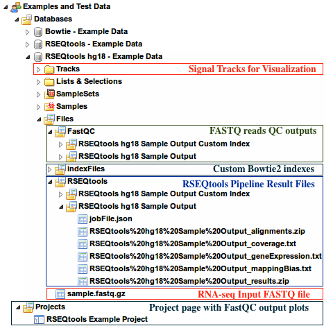
• Under the group Examples and Test Data, select the database RSEQtools hg18 - Example Data
• Input FASTQ file can be found under: Files » sample.fastq.gz
• Outputs of RSEQtools pipeline can be found under Files » RSEQtools folder of this database
• QC Plots from FastQC can be found in the Projects page
• Custom Bowtie2 indexes can be found under Files » indexFiles » bowtie » [Your custom index folder]
• Signal tracks are uploaded under the Tracks section of this database.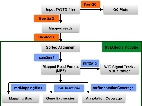

RSEQTools Pipeline - Workflow Implemented in the Genboree Workbench¶

1. Input Sequence import: User uploads single or paired-end FASTQ input sequence files to their database in the workbench
2. QC FastQ reads: Input FastQ sequence reads are checked for quality using FastQC
3. Map reads to reference genome: Sequence reads are mapped to reference genome using Bowtie 2
4. Sort alignments: Alignments in SAM format are sorted using Samtools
5. Convert to Mapped Read Format (MRF): Sorted Alignments in SAM format are converted to MRF using RSEQtools
6. Downstream analysis using modules in RSEQtools
   • Gene expression values: Calculate gene expression values using module mrfQuantifier
   • Annotation Coverage: Calculate annotation coverage value using module mrfAnnotationCoverage
   • Mapping Bias: Calculate mapping bias for a given annotation set using module mrfMappingBias
   • Signal Tracks: Generate signal tracks in WIG format using module mrf2wig

RSEQtools Modules used in Genboree Implementation¶

mrfQuantifier

This module calculates expression values (RPKM; read coverage normalized per million mapped nucleotides
and the length of the annotation model per kb). Given a set of mapped reads in MRF and an annotation set
(representing exons, transcripts, or gene models) mrfQuantifier calculates an expression value for each annotation entry.
This is done by counting all the nucleotides from the reads that overlap with a given annotation entry.
Subsequently, this value is normalized per million mapped nucleotides and the length of the annotation item per kb.

mrfMappingBias

Module to calculate mapping bias for a given annotation set. Aggregates mapped reads that overlap with
transcripts (specified in file.annotation) and outputs the counts over a standardized transcript
(divided into 100 equally sized bins) where 0 represents the 5' end of the transcript and
1 denotes the 3' end of the transcripts. This analysis is done in a strand specific way.

mrfAnnotationCoverage

Module to calculate annotation coverage. Sample a set of mapped reads and determine the
fraction of transcripts (specified in annotation file) that have at least -times uniform coverage.

mrf2wig

Generates signal track (WIG) of mapped reads from a MRF file. By default, the values in the
WIG file are normalized by the total number of mapped reads per million.
Only positions with non-zero values are reported.

References and Attributions¶

• Lukas Habegger, Andrea Sboner, Tara A. Gianoulis, Joel Rozowsky, Ashish Agarwal, Michael Snyder, Mark Gerstein.
  RSEQtools: A modular framework to analyze RNA-Seq data using compact, anonymized data summaries.
  Bioinformatics. 2010 Dec 5; 27(2) : 281-283 [PubMed]
• Langmead B, Salzberg SL. Fast gapped-read alignment with Bowtie 2. Nature Methods.
  2012 Mar 4; 9 : 357-359. [PubMed]
• Li H., Handsaker B., Wysoker A., Fennell T., Ruan J., Homer N., Marth G., Abecasis G., Durbin R. and
  1000 Genome Project Data Processing Subgroup. The Sequence alignment/map (SAM) format and SAMtools.
  Bioinformatics. 2009 25: 2078-9. [Pubmed]
• RSEQtools was developed by the Gerstein Lab
  at Yale University
• Integrated into the Genboree Workbench
  by Sai Lakshmi Subramanian
  at the Bioinformatics Research Laboratory, Baylor College of Medicine, Houston, TX.

Demo of small and long RNA-Seq pipelines at the ERCC 2nd Investigator's Meeting, May 2014¶

Live demos of small and long RNA-Seq pipeline given at the break-out sessions.

Date: Monday, May 19th, 2014.
Time: 10.35 a.m. and 3.15 p.m.
Location: Conf Room C

Presenters

Sai Lakshmi Subramanian – sailakss@bcm.edu (Primary Contact)
Kevin Riehle – riehle@bcm.edu
Bioinformatics Research Laboratory, Baylor College of Medicine, Houston, TX
Data Coordination Component (DCC) of exRNA Communication Consortium

Robert Kitchen - rob.kitchen@yale.edu
Department of Molecular Biophysics and Biochemistry, Yale University, New Haven, CT
Data Integration and Analysis Component (DiAC) of exRNA Communication Consortium

You can download a copy of the presentation in PDF format from here: Presentation

CIBR RNA-seq workshop - Demo of exceRpt small RNA processing pipeline, May 2015¶

Small RNA-Seq Data Analysis Tools in the Genboree Workbench

Date: Thursday, May 14th, 2015.
Time: 12.00 p.m. to 4.00 p.m.
Location: M321/323, DeBakey Building, Baylor College of Medicine

Presenter

Sai Lakshmi Subramanian (Primary Contact)
Bioinformatics Research Laboratory, Baylor College of Medicine, Houston, TX
Data Coordination Component (DCC) of exRNA Communication Consortium

Poster Presentation at the ISEV Annual Meeting , May 2016¶

ISEV Annual Meeting 2016

Dates: 4th-7th May, 2016
Location: Rotterdam, The Netherlands

Presenters

Rocco Lucero (Presenter at the Meeting)
Sai Lakshmi Subramanian
Bioinformatics Research Laboratory, Baylor College of Medicine, Houston, TX
Data Coordination Component (DCC) of exRNA Communication Consortium

DMRR Demo at the ERCC 3rd Investigator's Meeting, November 2014¶

Live demos of DMRR Data and Metadata Submission Infrastructure given at the break-out sessions.

Date: November 6th & 7th, 2014.

Presenters

William Thistlethwaite
Aaron Baker
Kevin Riehle
Sai Lakshmi Subramanian (Primary Contact)
Bioinformatics Research Laboratory, Baylor College of Medicine, Houston, TX
Data Coordination Component (DCC) of exRNA Communication Consortium

Robert Kitchen
Department of Molecular Biophysics and Biochemistry, Yale University, New Haven, CT
Data Integration and Analysis Component (DiAC) of exRNA Communication Consortium

DMRR Talk at the ERCC 5th Investigators' Meeting , November 2015¶

exRNA Profiling Data Submission & Analysis Infrastructure for the ERC Consortium

Date: November 9th, 2015 - Monday
Location: Rockville, MD

Presenters

Sai Lakshmi Subramanian
Bioinformatics Research Laboratory, Baylor College of Medicine, Houston, TX
Data Coordination Component (DCC) of exRNA Communication Consortium

• Introduction to Pathway and Interaction Analysis
• Target Interaction Finder
• Pathway Finder

Introduction to Pathway and Interaction Analysis¶

We have two different tools available on Genboree for pathway and interaction analysis.

The first, Target Interaction Finder, generates miRNA-protein target interaction files for a set of miRNA identifiers,
which can be imported into downstream tools, such as Cytoscape, for network analysis and visualization.

The second, Pathway Finder, performs a search for pathways either containing miRNAs of interest
or protein targets of those miRNAs.

You can visit each tool's tutorial page below.

Target Interaction Finder¶

You can view the tutorial page for the Target Interaction Finder tool here.

Pathway Finder¶

You can view the tutorial page for the Pathway Finder tool here.

• Using Pathway Finder to Perform a Search for Pathways Either Containing miRNAs of Interest or Protein Targets of Those miRNAs
• Introduction
• Instructional Video for Pathway Finder
• Preliminary Steps for Setting Up Any Analysis in the Genboree Workbench
• Create a Group for Your Analysis
• Create a Database for Your Analysis
• Upload your Data File(s)
• Step-by-step Instructions to Set Up Pathway Finder Submission
• Output Generated by Pathway Finder
• References and Attributions

Using Pathway Finder to Perform a Search for Pathways Either Containing miRNAs of Interest or Protein Targets of Those miRNAs¶

Introduction¶

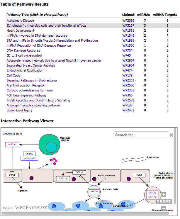
The Pathway Finder tool takes a column of miRNA identifiers from an input text file and performs a search for pathways either containing miRNAs of interest or protein targets of those miRNAs.
A table of pathway results and an interactive pathway viewer are displayed in an output window after the tool successfully processes the input text file.

Instructional Video for Pathway Finder¶

Below, you can view an instructional video for using the Pathway Finder Tool on the Genboree Workbench:

Preliminary Steps for Setting Up Any Analysis in the Genboree Workbench¶

Create a Group for Your Analysis¶

FAQ

What is a Group?

A "Group" contains Databases and Projects and controls access to all content within. You control access to your Group(s), and who is a member of your group. You can also belong to multiple Groups (i.e. collaborators).

This step is optional. You can also use your default/existing group.

Create a Database for Your Analysis¶

FAQ

What is a Database?

A "Database" contains Tracks, Lists, Sample Sets, Samples, and Files. Each database can be associated with a reference genome.

This step is optional.
Because this tool doesn't create any on-disk output, you only need to create a Database if you want to upload your own input file(s) for processing.
If you are using an input file in a previously existing Database (like the "Pathway Finder - Example Data" Database in the "Examples and Test Data" Group),
then you do not need to create a new Database.

If you do create a Database, make sure that you pick the proper reference sequence genome (hg19, for example) when creating your database.
Note that we do not have an entry for hg38 or mm10 in our "Reference Sequence" list.
If your data is associated with either of these reference sequence genomes, follow the directions below.

Create a Database for hg38 or mm10

In order to create a database associated with hg38 or mm10, select the "User Will Upload" option for "Reference Sequence"
and provide appropriate values for the Species and Version text boxes as given below:

Upload your Data File(s)¶

FAQ

Step-by-step Instructions to Set Up Pathway Finder Submission¶

1. Drag a single text file (with a first column consisting of miRNA identifiers) into the Input Data panel.
2. Select Visualization » Pathway Finder from the Toolset menu.
3. Click Submit. When we finish processing your input file, an output window will pop up with pathway results and an interactive pathway viewer.

Output Generated by Pathway Finder¶

After your input file is successfully processed, you will be able to view a table of pathway results and an interactive pathway viewer.
The first column of the table lists a clickable pathway title that updates the viewer.
The second column lists pathway identifers that link to WikiPathways.org.
The list is sorted by the number of "miRNAs" (primary) and by "miRNA Targets" (secondary) found on each pathway.
The top 20 results are listed.

References and Attributions¶

1. WikiPathways, source for curated pathways and miRNA content: Pico AR, et al. (2008) WikiPathways: Pathway Editing for the People. PLoS Biol 6(7). http://journals.plos.org/plosbiology/article?id=10.1371/journal.pbio.0060184
2. miRTarBase source database for experimentally validated miRNA-protein target interactions: Chou et al. miRTarBase 2016: updates to the experimentally validated miRNA-target interactions database. NAR, Database Issue, Vol 44(D1). http://www.ncbi.nlm.nih.gov/pmc/articles/PMC4702890/
3. Pathway Finder tool was designed and implemented by Anders Riutta and Alexander Pico, and the video tutorial was produced by Kristina Hanspers, all at the Gladstone Institutes, San Francisco, CA.
4. Integrated into the Genboree Workbench by William Thistlethwaite at the Bioinformatics Research Laboratory, Baylor College of Medicine, Houston, TX.

This tool has been deployed in the context of the exRNA Communication Consortium (ERCC).
Please contact William Thistlethwaite with questions or comments, or for help using it on your own data.

• Small RNA-Seq Data Analysis for exRNA Profiling Using the exceRpt Small RNA-seq Pipeline
• Version Updates
• Preliminary Steps for Setting Up Any Analysis in the Genboree Workbench
• Create a Group for Your Analysis
• Create a Database for Your Analysis
• Upload your Data File(s)
• Step-by-step Instructions for Setting Up Your exceRpt small RNA-Seq Data Analysis
• Notes for Preparing Input Data Files
• Tool Settings
• Example Data for Running exceRpt Small RNA-seq Pipeline
• exceRpt Small RNA-seq Pipeline Workflow (Implemented in the Genboree Workbench)
• exRNA Data Analysis Results
• Currently Supported Genomes
• Sources of smallRNA Libraries
• Workflow
• Example of Core Results from Workflow
• Post-processing of Samples
• Explanation of Exogenous Output
• Example of Post-processed Result Files
• Comparative Plots
• Bioinformatics Tools Used in This Pipeline (4th Gen)
• References and Attributions

Small RNA-Seq Data Analysis for exRNA Profiling Using the exceRpt Small RNA-seq Pipeline¶

Version Updates¶

Current version: v4.6.2 (as of 10/12/2016)

The newest version of exceRpt is 4.6.2, which contains many updates compared to the previous, 3rd generation version on Genboree (3.3.0).
We currently still give users the option to run jobs using 3rd gen. exceRpt.
Note that some images below may have slightly outdated version numbers, but the content of the images remains otherwise accurate.

To read more about recent updates to exceRpt, view the Version Updates.

Preliminary Steps for Setting Up Any Analysis in the Genboree Workbench¶

Create a Group for Your Analysis¶

FAQ

What is a Group?

A "Group" contains Databases and Projects and controls access to all content within. You control access to your Group(s), and who is a member of your group. You can also belong to multiple Groups (i.e. collaborators).

This step is optional. You can also use your default/existing group.

Create a Database for Your Analysis¶

FAQ

What is a Database?

A "Database" contains Tracks, Lists, Sample Sets, Samples, and Files. Each Database can be associated with a reference genome.

This step is required.
You can leave "Species" and "Version" blank, as those fields are not used by exceRpt.
You can also leave "Reference Sequence" as "** User Will Upload **" - exceRpt uses its own reference files, so it doesn't need to consult your Database's reference sequence.
You will receive a warning message when creating your Database - just ignore this warning and proceed.

Upload your Data File(s)¶

FAQ

Step-by-step Instructions for Setting Up Your exceRpt small RNA-Seq Data Analysis¶

1. Drag one or more archives containing single-end FASTQ or SRA files to the Input Data panel. The input file(s) must be compressed.
   Each FASTQ/SRA file can also be compressed inside these archives.
   Check out the Notes below for more info on preparing your input data files.
2. Drag a Database to the Output Targets panel to store results.
3. Select Transcriptome » Analyze Small RNA-Seq Data » exRNA Data Analysis » exceRpt small RNA-seq Pipeline from the tool menu.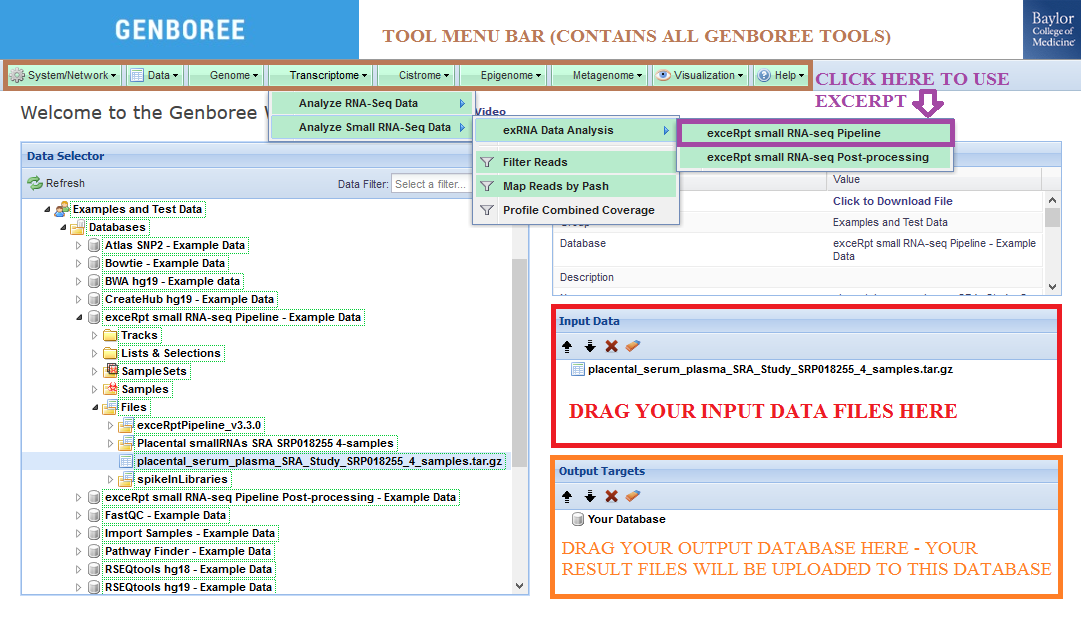
   
4. Fill in appropriate details in the Tool Settings dialog box. See Tool Settings for more details.
5. Submit your job. You will receive several emails as we process your samples.
   • First, you will receive an email about your exceRpt small RNA-seq Pipeline (New, Customized Endogenous Engine) Batch Submission job.
     This email just lets you know if your samples were successfully submitted for processing.
   • Second, you will receive one or more emails about your Run exceRpt on Single Sample job(s).
     You will receive an email for each sample submitted, and those emails will let you know which samples were processed successfully.
     If you selected the "Suppress Individual Sample Emails" option, you will not receive these emails.
   • Third, you will receive an email about your Generate Summary Report for exceRpt Results job.
     This email lets you know if post-processing on your samples was performed successfully.
   • Fourth, you will receive an email about your ERCC Final Processing job.
     This email will give you a brief summary report about the different jobs above.
6. Download the results of your analysis from your Database. The results data will end up under the exceRptPipeline_v4.6.2 folder in the Files area of your output Database.
   • Within that folder, your Analysis Name will be used as a sub-folder to hold the files generated by that run of the tool.
   • In order to see the results for a particular sample, open the sub-folder corresponding to that sample.
   • If you selected the "Upload Full Results" option, you will see a results .zip that will contain all result files from your exceRpt run, including any full alignment .bam files.
     • Click on the results archive (.zip) in the Data Selector panel.
     • Select the link Click to Download File from the Details panel to download the results archive.
   • The .stats file will contain the read counts mapped at various stages of the exceRpt mapping process.
   • Open the CORE_RESULTS sub-folder to download the CORE_RESULTS archive (.tgz). This archive contains the most important files from your exceRpt run.
     • This archive is usually all you need from a given exceRpt run and is much smaller than the full results archive (.zip) since it doesn't contain full alignment .bam files.
     • The CORE_RESULTS archive will be decompressed in the CORE_RESULTS folder on the Workbench for your convenience.
   • Finally, under the Analysis Name folder, you will also find a sub-folder named postProcessedResults_v4.6.3 that contains post-processing results and plots for all of your submitted samples.
     • These files are described in further detail below.

Notes for Preparing Input Data Files¶

RECOMMENDATION:

• If you have a large number of input FASTQ/SRA files, it is highly recommended to make smaller archives with fewer numbers of input files
  in order to avoid issues with uploading the archives to your Genboree Database.
  • Each compressed archive should be smaller than 10GB.
  • Upload all of your smaller archives to your Genboree Database and then submit them all in the same exceRpt Small RNA-seq Pipeline job.
  • This technique will allow you to successfully upload many input files and compare/contrast results from those input files in one job submission.

IMPORTANT NOTES:

• The archive should not contain any folders or sub-folders - all files should be directly placed into the archive.
  If you are using Mac OS to prepare your files, remember to remove the "__MACOSX" sub-directory that gets added to the compressed archives.
• In order to create your archive using the terminal, first navigate to the directory where your files are.
  • EXAMPLE: If my files were located in C:/Users/John/Desktop/Submission, I would use the "cd" command in my terminal and type
    

    cd C:/Users/John/Desktop/Submission
    

  • Next, you will use the zip command with the -X parameter (to avoid saving extra file attributes) to compress your files.
  • EXAMPLE: Imagine that I am submitting 4 data files : inputSequence1.fq.gz, inputSequence2.fq.bz2, inputSequence3.fq.zip, inputSequence4.sra
    I want to name my .zip file johnSubmission.zip
    • I would type the following:
      

      zip -X johnSubmission.zip inputSequence1.fq.gz inputSequence2.fq.bz2 inputSequence3.fq.zip inputSequence4.sra
      

• Commonly used compression formats like .zip, .gz, .tar.gz, .bz2 are accepted.

Tool Settings¶

• exceRpt Version You can choose between using 4th gen exceRpt (4.6.2) and 3rd gen exceRpt (3.3.0) here.
  Only settings relevant to the chosen version of exceRpt will be displayed.
  We will remove the option to use 3rd gen exceRpt in the near future.
• Analysis Name This name is used under the top-level output folder (exceRptPipeline_v4.6.2) in order to organize your processed pipeline results.
  You should include identifying information (timestamp, disease associated with samples, etc.) in your analysis name so you can easily distinguish between your different submissions.
• Genome Version You can choose the genome version associated with your input files here. Please note that only one genome version is allowed per submission.
• ERCC Submission Options Here, if you are a member of the ERCC, you can select the grant number and anticipated data repository associated with your submission.
  If your submission does not fall under an ERCC grant, then choose the 'Non-ERCC Funded Study' option.
  If you are an ERCC member and your PI / grant numbers are not showing up properly, please email exRNA Team with your PI's name so you can be added to our database as a submitter.
• 3' Adapter Sequence Options You can select your 3' adapter sequence here. By default, we will attempt to auto-detect the adapter sequence for your samples.
  Auto-detection is a good choice if you don't know your 3' adapter sequence or if your submission includes samples with different 3' adapter sequences,
  as we don't currently support manual input of multiple 3' adapter sequences in the same submission.
  You can also select one of the pre-defined 3' adapter sequences, manually specify your own 3' adapter sequence, or select the NO 3' ADAPTER option if your samples have already had their 3' adapters clipped.
• Random Barcode Options If your sequences have adapter sequences that contain short random barcodes, click the Random Barcodes Present in Samples? checkbox.
  You'll then be able to enter the length and location of your random barcodes.
  The exceRpt pipeline can also compute frequency and enrichment statistics for samples with random barcodes.
  Such metrics can be useful in some circumstances for identifying ligation/amplification biases in smallRNA samples.
  Click the Compute Barcode Stats checkbox to enable this option. Choosing this option will make your job run more slowly.
• Advanced Preprocessing Options (initially minimized)
  • Trim Bases on 3p End - This option will trim N bases from the 3' end of each read, where N is the value you choose. Default of 0.
  • Trim Bases on 5p End - This option will trim N bases from the 5' end of each read, where N is the value you choose. Default of 0.
  • Minimum Read Length - This option will alter the minimum read length we will use after adapter (and random barcode) removal. Minimum value allowed is 10. Default of 18.
  • Minimum Base-call Quality of Reads - This option will alter the minimum base-call quality of reads. Default of 20.
  • Percentage of Read That Must Meet Minimum Base-call Quality - This option will alter the percentage of a given read that must meet the minimum base-call quality given above. Default of 80.
• Oligo (Spike-in) Library Options - There are 3 options:
  • No custom oligo library - No mapping to custom oligo library.
  • Upload new custom oligo library - Upload a single FASTA file with a list of all spike-in sequences used.
    Uploaded sequences are stored under the Files » spikeInLibraries sub-folder in your Database for future use.
  • Use existing oligo library - Select an existing oligo library from your Database.
• Endogenous Alignment Options
  • You can select your order of preference for endogenous library alignment.
    • Numbers are listed in order of priority ('1' is higher priority than '2', etc.).
    • By default, the quantification engine will first align to miRNA, then tRNA, then pIRNA, then Gencode annotations, and then circular RNA.
    • You can change the order of priority by altering the numbers next to each library.
    • If you do not want to align to a particular library, erase the number for that particular library. You may also use the "Remove" buttons.
    • You may not choose the same priority for multiple libraries.
• Advanced Endogenous Alignment Options (initially minimized)
  • Maximum Number of Endogenous Mismatches Allowed - This option will alter the maximum number of mismatches allowed during endogenous alignment. Range from 0 to 3. Default of 1.
  • Minimum Fraction of Read Remaining After Soft Clipping - This option will alter the minimum fraction of the read that must remain following soft-clipping (in a local alignment). Default of 0.9.
  • Downsample RNA Reads for Transcriptome Alignments - This option will allow you to downsample your RNA reads after assigning reads to the various transcriptome libraries.
    This may be useful for normalizing very different yields. If you want to downsample, click the checkbox and then put the number of RNA reads to which you want to downsample.
    We recommend a minimum of 100000, which is the default if you choose to downsample.
• Exogenous Alignment Options
  • You can select your preference for exogenous library alignment. There are three options:
    • Endogenous-only - Disables mapping to exogenous miRNAs.
    • Endogenous + exogenous (miRNA) - Maps to exogenous miRNAs in miRBase (i.e., from plants and viruses).
    • Endogenous + exogenous (miRNA + Genome) - Maps to exogenous miRNAs in miRBase AND the genomes of all sequenced species in Ensembl/NCBI.
    • Note that if you choose either the second or third option, then you cannot turn off any of the endogenous mappings above.
    • If you have already turned off any endogenous mappings, then you cannot choose either the second or third option.
• Advanced Exogenous Alignment Options (initially minimized)
  • Maximum Number of Exogenous Mismatches Allowed - This option will alter the maximum number of mismatches allowed during exogenous alignment. Range from 0 to 1. Default of 0.
• Other Advanced Options (initially minimized)
  • Remote Storage Area - This option will allow you to choose a remote storage (FTP) area where your result files will be uploaded.
    These result files will then be accessible via FTP client. You can learn more by visiting the Using Remote (FTP) Storage for exceRpt help page.
  • Suppress Individual Sample Emails - This option will turn off the individual runExceRpt emails for each sample as it gets processed.
    If your submission includes dozens of samples and you'd prefer to not receive dozens of emails, click the checkbox.
  • Upload Full Results - This option will upload all of the result files for each sample, as opposed to the core, most important files that are normally uploaded.
    For example, a full results archive will contain all of the full alignment .bam files generated by the pipeline.
    This archive will be much larger than the core results archive and will significantly eat into your allotted storage space, so only select this option if necessary!
    To learn more about the storage quotas we have recently implemented, view the Understanding Your Storage Options with exceRpt page.

Example Data for Running exceRpt Small RNA-seq Pipeline¶

In this example, we have used four samples from deep sequencing experiments of barcoded small RNA cDNA libraries to profile microRNAs in
cell-free serum and plasma from human volunteers. These samples were analyzed using the exceRpt Small RNA-seq Pipeline.

The sample input FASTQ files and output results and plots can be found here:

• Under the group Examples and Test Data, select the Database exceRpt small RNA-seq Pipeline - Example Data.
• The compressed input files can be found in the archive: Files » placental_serum_plasma_SRA_Study_SRP018255_4_samples.tar.gz.
  • These same compressed input files can be found unarchived in the following folder: Files » Placental smallRNAs SRA SRP018255 4-samples.
• Pipeline results can be found under the Files » exceRptPipeline_v4.6.2 » Circulating microRNAs from serum plasma - Study SRP18255 folder.
  • Each sample has its own dedicated folder (sample_C1_non_pregnant1_SRR822433_fastq, sample_C3_non_pregnant3_SRR822434_fastq, etc.).
• Core result files for a given sample can found in its CORE_RESULTS folder.
• Post-processing plots and results for all samples can be found in the postProcessedResults_v4.6.3 folder (under the Circulating microRNAs from serum plasma - Study SRP18255 folder).

exceRpt Small RNA-seq Pipeline Workflow (Implemented in the Genboree Workbench)¶

The exceRpt Small RNA-seq Pipeline is for the processing and analysis of RNA-seq data generated to profile small-exRNAs.
The pipeline is highly modular, allowing the user to define the libraries containing smallRNA sequences that are used
during RNA-seq read-mapping, including an option to provide a library of spike-in sequences to allow absolute quantitation
of small-RNA molecules. It also performs automatic detection and removal of 3' adapter sequences.

The output data includes abundance estimates for each of the requested libraries, a variety of quality control metrics
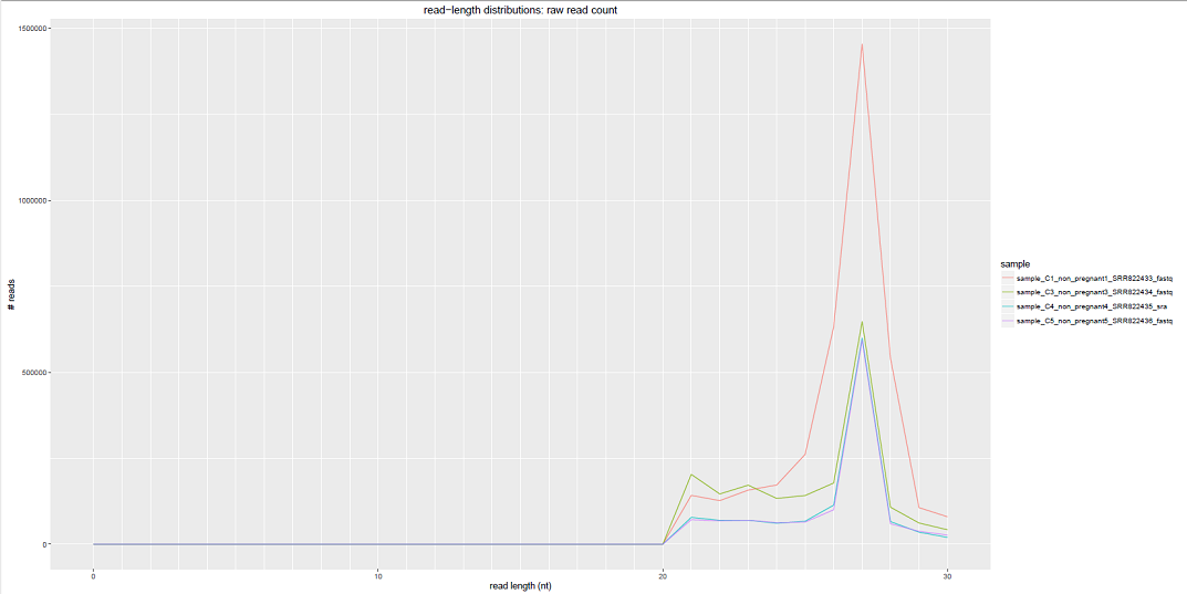
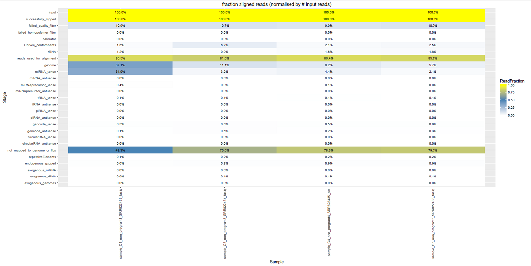
such as read-length distribution, summaries of reads mapped to each library, and detailed mapping information for each read mapped to each library.

exRNA Data Analysis Results¶

To better understand the results generated by exceRpt, check out the exRNA Data Analysis page.

Finally, after the pipeline finishes processing all submitted samples, a separate post-processing tool (processPipelineRuns)
is run on all successful pipeline outputs. This tool generates useful summary plots and tables that can be used to compare
and contrast different samples.

Currently Supported Genomes¶

• Human Genome version - hg38
• Human Genome version - hg19
• Mouse Genome version - mm10

Sources of smallRNA Libraries¶

• rRNAs from 45S, 5S, and mt_rRNA sequences for human and mouse
• miRNAs from miRBase version 21
• tRNAs from gtRNAdb
• piRNAs from piRNABank (removed duplicate sequences)
• Annotations from Gencode version 24 (hg38), version 18 (hg19), version M9 (mm10)
• CircularRNAs from circBase

Workflow¶

Example of Core Results from Workflow¶

Post-processing of Samples¶

After all samples have been processed through this pipeline, the Generate Summary Report for exceRpt Results tool will take
successful samples and perform post-processing on them.

This post-processing step will generate useful plots and tables that will allow you to compare and contrast samples.
A description of all generated files can be found in the table below (partially taken from the exceRpt GitHub page):

Explanation of Exogenous Output¶

The taxonomy specific read counts file contains the number of reads that map directly to each node in the sample's taxonomy tree.
The taxonomy cumulative read counts file contains the number of reads that map to the descendants of each node in the sample's taxonomy tree.
Importantly, the reads counted for a given node in the taxonomy specific read counts file are NOT counted as part of the cumulative counts in the other file
(all of the node's descendants are counted, but not the node itself).

• 1 superkingdom 10239 1 Viruses 131 182 141 15 122 136 97 100 115

• 1 superkingdom 10239 1 Viruses 0 0 0 0 0 0 0 0 0

This means that no reads mapped directly to the Viruses node, but a considerable number of reads mapped to descendants of Viruses.

• 1 no rank 131567 1 cellular organisms 649526 737020 724361 200600 316643 412608 365094 374525 473008

• 1 no rank 131567 1 cellular organisms 791672 806489 734921 211454 320147 398621 348969 407637 494698

This means that a considerable number of reads mapped both directly to the cellular organisms node as well as descendants of that node.

In other words, if you want to get a full count of all of the reads that aligned to a given node and its descendants,
you need to ADD TOGETHER the numbers in both the taxonomy cumulative and taxonomy specific files for that node.

You can also find plots of the exogenous trees in the .pdf plot files.
First, the TaxonomyTrees_perSample.pdf file contains a plot for each sample.
The percentage within each node is the ratio of the node's summed cumulative + specific reads to the root node's summed cumulative + specific reads.
Second, the TaxonomyTrees_aggregateSamples.pdf file contains a single plot that condenses all samples into a single, averaged tree.
The percentage within each node is the ratio of that node's summed cumulative + specific reads averaged across all samples to the root node's summed cumulative + specific reads averaged across all samples.

Example of Post-processed Result Files¶

Below, we can see what the post-processing files look like on the Genboree Workbench (found in the Examples and Test Data Group):

Comparative Plots¶

We can see some examples below of the comparative plots available in the DiagnosticPlots.pdf generated by the post-processing tool.
Each plot contains data from four different samples (the example data).

Bioinformatics Tools Used in This Pipeline (4th Gen)¶

• FASTX-Toolkit v0.0.14
• Bowtie2 v2.2.6
• Samtools v1.3.1
• SRA-Toolkit v2.3
• R v3.2
• FastQC v0.11.2
• STAR v2.4.2a

References and Attributions¶

• This tool has been developed by the Data Integration and Analysis Component (DIAC) of the Extracellular RNA Communication Consortium
• exceRpt small RNA-seq pipeline was developed by Robert Kitchen at the Gerstein Lab at Yale University
• Dobin A, Davis CA, Schlesinger F, et al. STAR: ultrafast universal RNA-seq aligner. Bioinformatics. 2013;29(1):15-21. doi:10.1093/bioinformatics/bts635. [Pubmed]
• Kozomara A, Griffiths-Jones S. miRBase: integrating microRNA annotation and deep-sequencing data. NAR 2011 39 (Database Issue):D152-D157 [Pubmed]
• Langmead B, Salzberg SL. Fast gapped-read alignment with Bowtie 2. Nature Methods. 2012 Mar 4; 9 : 357-359. [PubMed]
• Integrated into the Genboree Workbench by Sai Lakshmi Subramanian and William Thistlethwaite
  at the Bioinformatics Research Laboratory, Baylor College of Medicine, Houston, TX.

This tool has been deployed in the context of the exRNA Communication Consortium (ERCC).
Please contact "exRNA Team":brl-exrna@bcm.edu with questions or comments, or for help using it on your own data.

• Generating miRNA-Protein Target Interaction Files for a Set of miRNA Identifiers Using Target Interaction Finder
• Introduction
• Instructional Video for Target Interaction Finder
• Preliminary Steps for Setting Up Any Analysis in the Genboree Workbench
• Create a Group for Your Analysis
• Create a Database for Your Analysis
• Upload your Data File(s)
• Step-by-step Instructions to Set Up Target Interaction Finder Submission
• Output Files Generated by Target Interaction Finder
• References and Attributions

Generating miRNA-Protein Target Interaction Files for a Set of miRNA Identifiers Using Target Interaction Finder¶

Introduction¶

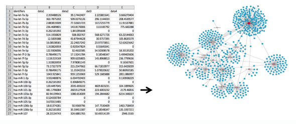
This tool takes a column of miRNA identifiers from an input TXT file and generates miRNA-protein target interaction files in both a tabular CSV format and a network XGMML format.
The target interactions are sourced from miRTarBase ¹, an experimentally validated miRNA-target interaction database.
The CSV and XGMML files can be imported into downstream tools, such as Cytoscape ², for network analysis and visualization.

From a column of identifiers... to a network of interactions

Instructional Video for Target Interaction Finder¶

Below, you can view an instruction video for using the Target Interaction Finder Tool on the Genboree Workbench:

Preliminary Steps for Setting Up Any Analysis in the Genboree Workbench¶

Create a Group for Your Analysis¶

FAQ

What is a Group?

A "Group" contains Databases and Projects and controls access to all content within. You control access to your Group(s), and who is a member of your group. You can also belong to multiple Groups (i.e. collaborators).

This step is optional. You can also use your default/existing group.

Create a Database for Your Analysis¶

FAQ

What is a Database?

A "Database" contains Tracks, Lists, Sample Sets, Samples, and Files. Each database can be associated with a reference genome.

This step is required.
Make sure that you pick the proper reference sequence genome (hg19, for example) when creating your database.
Note that we do not have an entry for hg38 or mm10 in our "Reference Sequence" list.
If your data is associated with either of these reference sequence genomes, follow the directions below.

Create a Database for hg38 or mm10

In order to create a database associated with hg38 or mm10, select the "User Will Upload" option for "Reference Sequence"
and provide appropriate values for the Species and Version text boxes as given below:

Upload your Data File(s)¶

FAQ

Step-by-step Instructions to Set Up Target Interaction Finder Submission¶

1. Drag one or more text files (each with a first column consisting of miRNA identifiers) into the Input Data panel. These input file(s) can also be compressed, as mentioned above.
2. Drag a Database to the Output Targets panel to store results.
3. Select Visualization » Target Interaction Finder from the Toolset menu.
4. Fill in the analysis name for your tool job. We recommend keeping a timestamp in your analysis name!
5. Submit your job. Upon completion of your job, you will receive an email.
6. Download the results of your analysis from your Database. The results data will end up under the targetInteractionFinder folder in the Files area of your output database.
   • Within that folder, your Analysis Name will be used as a sub-folder to hold the files generated by that run of the tool.
   • Open this sub-folder to see your results.
   • Select any of the output files (explained in more detail below) and then click the link Click to Download File from the Details panel to download that output file.

Output Files Generated by Target Interaction Finder¶

After your job successfully completes, you will be able to download 3 different output files:

• A .csv file that contains the following columns:
  1. queryid – the miRNA identifiers provided in the input file
  2. targeted – the protein identifier provided by miRTarBase, i.e., Entrez Gene
  3. pmid – pubmed identifier for article of evidence for interaction
  4. datasource – name of source database of miRNA-protein targets
• A .xgmml file that contains many annotations on both miRNA and protein nodes as well as on the interactions themselves.
  • This file can be imported natively into network software tools such as Cytoscape.
• A summary.log file that contains summary information about the interactions found in the files above.

References and Attributions¶

1. miRTarBase source database for experimentally validated miRNA-protein target interactions: Chou et al. miRTarBase 2016: updates to the experimentally validated miRNA-target interactions database. NAR, Database Issue, Vol 44(D1). http://www.ncbi.nlm.nih.gov/pmc/articles/PMC4702890/
2. Cytoscape tool for network visualization and analysis: Shannon, P, et al. Cytoscape: a software environment for integrated models of biomolecular interaction networks. Genome Research, 13(11). http://genome.cshlp.org/content/13/11/2498.full
3. Target Interaction Finder tool written by Anders Riutta and Alexander Pico at the UCSF Gladstone Institute, San Francisco, CA.
4. Integrated into the Genboree Workbench by William Thistlethwaite and Sai Lakshmi Subramanian at the Bioinformatics Research Laboratory, Baylor College of Medicine, Houston, TX.

This tool has been deployed in the context of the exRNA Communication Consortium (ERCC).
Please contact William Thistlethwaite with questions or comments, or for help using it on your own data.

• Understanding Your Storage Options with exceRpt
• Basics on Storage Quotas
• What Files Contribute to Your Quotas?
• Recommendations for Meeting the Quotas
• Deleting Files
• Compressing Files
• Moving Files to Different Storage Type
• Requesting More Space for Your Group

Understanding Your Storage Options with exceRpt¶

We have recently implemented some storage quotas for using exceRpt.
In particular, these quotas apply when you select the "Upload Full Results" option.
Please read the information below to better understand the storage quotas
and how you can clear up space for your Genboree Group.

Basics on Storage Quotas¶

Each Genboree Group has two different storage quotas associated with it.
These storage quotas include local space and FTP-backed space.
Note that the quotas are associated with a Group and not a user!
Please do not create multiple Groups as a single user to bypass the quota restriction.
You should only use a single Group for your exceRpt output (unless discussed with us previously).

By default, a Genboree Group is allotted 100 GB of local space and 100 GB of FTP-backed space.
Local space is defined as any space outside of the virtual FTP areas in your Group.
You can learn more about creating virtual FTP areas on the Workbench here.

As mentioned above, these space requirements only apply if you launch an exceRpt job with
the "Upload Full Results" option enabled. This option will upload a large results archive for each
sample containing alignment .bam files (and other similar files).
You can learn more about the specific files present in the full results archive on the exRNA Data Analysis page.

The default storage quotas should be sufficient for most users, especially if you normally run your samples
through exceRpt without the "Upload Full Results" option.

What Files Contribute to Your Quotas?¶

Any files in your Genboree Group will contribute to either the local or FTP-backed quota.
For example, if I uploaded a large number of FASTQ files that I wanted to process, those would contribute to one of the quotas.
This is one reason why it is very important to compress your files on the Workbench.
You can learn more about this idea below.

When you submit your files for processing through exceRpt (with "uploadFullResults" enabled),
the following factors will be considered:

1) How much space you're currently taking up in your Group (discussed above)
2) An estimation of how much space your current submission will take up when fully uploaded
3) An estimation of how much space your other, currently-running submissions will take up when fully uploaded

In other words, if I launch a huge job with 200 samples, I will likely get an error message when I try to launch another job,
even if my first job hasn't finished yet.

If you do receive an error message, it will clearly indicate how much space is taken up by each of the enumerated factors above.

Recommendations for Meeting the Quotas¶

Because we only recently instituted these quotas, many Genboree Groups have far exceeded the numbers given above
and cannot launch exceRpt jobs until space is freed up.
We have a number of suggestions for meeting the quotas:

Deleting Files¶

If you have any files that you no longer need on the Workbench, you can delete those files to free up space.
You should use the Remove File(s) tool (found under Data -> Files) to do so.
Simply drag your files into the Input Data panel and then run the tool to delete them.
The tool also accepts folders as inputs, so if you want to delete an entire folder at once, you can do that also.
Remember that exceRpt is constantly being worked on and improved, so if you have some old results, you could
potentially delete those and re-run your samples through the newest version of exceRpt.

Compressing Files¶

Another way to make space is to compress your files if they are currently uncompressed.
For example, many users have uncompressed FASTQ files stored on Genboree.
These FASTQ files can be very large, but they get much smaller when they're compressed.

Furthermore, we recently added a restriction to exceRpt so that it no longer accepts uncompressed FASTQ files as input.
This means that if you want to use FASTQ files in exceRpt, you will need to compress them first.
You can compress the files on the Genboree Workbench using the Prepare Archive tool (found under Data -> Files).
Simply drag your uncompressed files into the Input Data panel and the Database where you want your archive created
into the Output Targets panel.

IMPORTANT: After you run the tool and receive an email informing you that the job was successful,
you must manually delete your old uncompressed files. We will implement an option in the near future
that will do this deletion automatically, but for now, you'll need to do it using the Remove File(s) tool (discussed above).

Moving Files to Different Storage Type¶

As mentioned above, we have two different quotas: one for local storage and one for FTP-backed storage.
Thus, if one quota is completely full, it might make sense to move some files to a different storage type to free up space.
You can accomplish this by using the "Copy / Move File" tool (found under Data -> Files).
In most cases, users will want to move their files from local storage to FTP-backed storage, so we'll explain how to do that below.

1. Create a virtual FTP area if you haven't already. You can follow the directions here.
2. Drag the files you want to move into the Input Data panel.
3. Drag the folder associated with the virtual FTP area into the Output Targets panel.
4. Use the Copy/Move File tool and select the MOVE option (we do not want to copy the files).

If you do have files in your FTP-backed area that you want to move to local storage, the method is very similar.
Drag the files you want to move into the Input Data panel, and then drag the Database where you want your files to be stored
into the Output Targets panel.

Requesting More Space for Your Group¶

Before requesting more space, you should try all of the methods given above.
If you still need more space, email Emily and let him know your Genboree Group and why you need more space.
For example, if your Group stores files associated with a collaborative effort between several different labs,
then it might make sense to increase that Group's storage quota.

• Using Remote (FTP) Storage for exceRpt
• Step 1: Creating Your Remote Storage Area
• Step 2: Submitting Your Samples to exceRpt
• Step 3: Accessing Your Results
• Accessing Your Results via the Genboree Workbench
• Accessing Your Results via Your FTP Client

Using Remote (FTP) Storage for exceRpt¶

• Files are still accessible via Genboree Workbench, but they are also accessible via FTP client
• Downloading via FTP client is more reliable for large files - you can even resume your downloads!

Below, we'll go step-by-step through the process of setting up your remote storage area on Genboree and then downloading your exceRpt result files.

Step 1: Creating Your Remote Storage Area¶

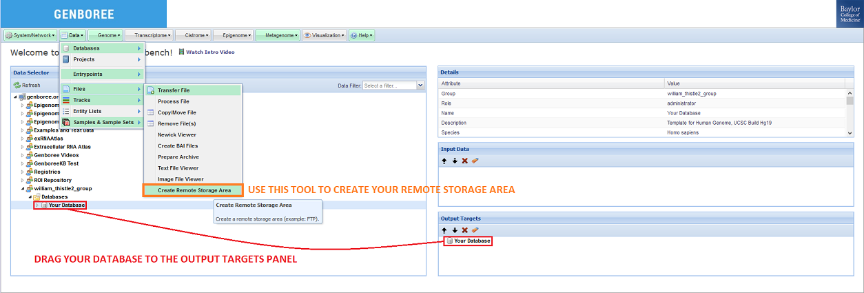
The first step in the process is creating a remote storage area in your Database of choice.
If you're unfamiliar with Genboree, you should first learn about Groups and then learn about creating Databases.
Note that your account comes with a default group named after your user login.

After you have created a Database, you should drag it from the Data Selector panel to the Output Targets panel.
Then, you can select the Create Remote Storage Area tool in the tool menu at the top of the screen:

When you click the Create Remote Storage Area button, a window like the following will appear:

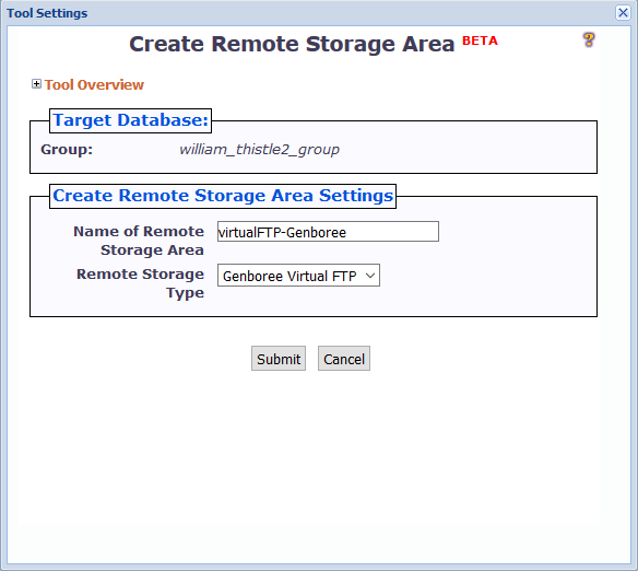
There are two different settings you can change:

1. Name of Remote Storage Area
2. Remote Storage Type

You can name the remote storage area anything you want, so long as the name is unique among folders in the Files area of your Database.
This is because the remote storage area is represented as a folder in the Files area.

Under "Remote Storage Type", you can select the particular type of remote storage area that you want to create.
Currently, we only support the Genboree FTP server - thus, you can go ahead and keep the default option of "Genboree Virtual FTP".

After you click "Submit", you will receive notification that your remote storage area was successfully created (or an informative error message if something went wrong).
Your remote storage area will now be available in the Files area under the Database you chose:

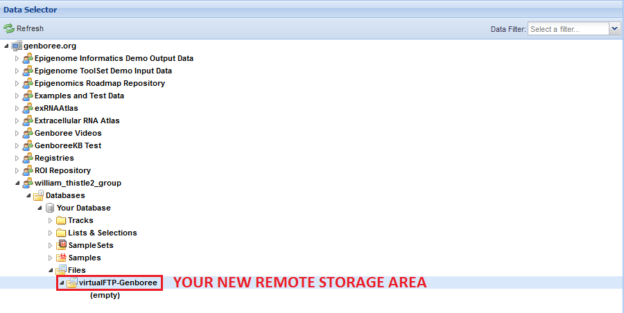
You can use this tool to create as many remote storage areas as you like, so long as they all have different names.

Step 2: Submitting Your Samples to exceRpt¶

Now that you've created your remote storage area, the next step is to submit your files for processing through exceRpt.
This tutorial will provide guidance on submitting your samples.
In particular, you will need to select your newly created remote stage area in the Remote Storage Area menu under Advanced Options.
The default option for this menu is None Selected - you should choose the remote storage area where you want to store your exceRpt result files.

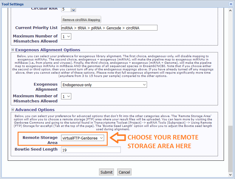
After you click "Submit", your files will be processed through exceRpt.
If any issue arises during processing, you will receive an email notifying you about the issue.
If you have additional questions about your submission, you can always email exRNA Team for help.

Step 3: Accessing Your Results¶

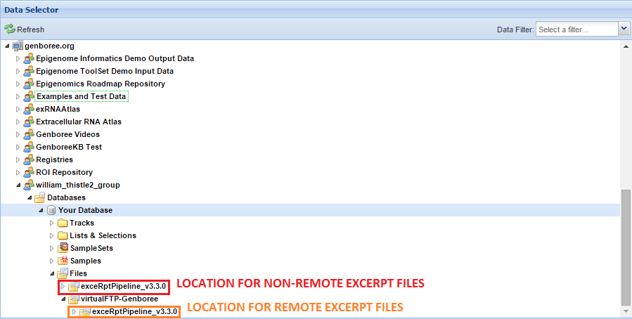
After we've finished processing your samples, you'll be able to access your results by both the Genboree Workbench and your FTP client.

Accessing Your Results via the Genboree Workbench¶

If you want to use the Genboree Workbench, accessing your samples is just like any other exceRpt job, with one small difference.
With normal exceRpt submissions, the base directory for your exceRpt pipeline runs can be found in the Files area.
However, if you use a remote storage area, the base directory for your exceRpt pipeline runs will be located in that remote storage folder.
You can see an example below:

Accessing Your Results via Your FTP Client¶

Before you can access your results, you will need an account on our FTP server.
You should email exRNA Team and ask her to create a personal FTP account for you so that you can log onto our FTP server.
Please note that creating a Genboree account does not create your FTP account as well.
You will always need to contact the exRNA Team in order to create your FTP account.

1. Your Genboree username. Ex: william_thistle
2. Your Group name. Ex: william_thistle2_group
3. The name of the database which contains the remote storage area.
4. The name of the remote storage area you created following the above instructions so we know which folder to give FTP access. Ex: virtualFTP-Genboree
5. The PI name. This is important if you will be doing data submissions. Ex: Dr. Milosavljevic

Note: If you would like multiple people to have download permissions for this FTP folder you can include the usernames of the other people here

• /genboree:genboree.org/william_thistle2_group/Your_Database/virtualFTP-Genboree/exceRptPipeline_v3.3.0/
  • Note that "Your Database" has been escaped so it's now "Your_Database".

Please note that you must send an email to us for each new Database you want to use for remote storage.
For example, say you create a remote storage area in Database A and then ask us to expose that area to your FTP username.
We will do so, and then you will be able to see that area via your FTP client.
If you create more remote storage areas in the same Database (Database A), then you will also be able to see those areas without emailing us again.
However, if you create a new Database on Genboree (Database B) and then create a remote storage area in that Database,
you will need to email us again with the name of the new Database so we can expose it to your FTP username.

• exceRpt Small RNA-seq Data Analysis Pipeline - +Version Updates+
• 4th Generation
• v4.6.3 (Version available on GitHub)
• v4.6.2 (Version associated with exRNA Atlas and currently available on Genboree Workbench)
• v4.4.1 through v4.6.1
• v4.3.1 through v4.4.0
• v4.2.0 through v4.3.0
• v4.1.0 through v4.1.9
• v4.0.0 through v.4.0.9
• 3rd Generation
• v3.4.1 (not installed on Genboree)
• v3.4.0 (not installed on Genboree)
• v3.3.0 (Version associated with exRNA Atlas v3 Snapshot)
• v3.2.6
• v3.1.9
• v3.1.5
• v3.1.1
• 2nd Generation (Discontinued)
• v2.2.8
• v2.2.6
• v2.2.2
• v1.3.3
• v1.0

exceRpt Small RNA-seq Data Analysis Pipeline - Version Updates¶

4th Generation¶

v4.6.3 (Version available on GitHub)¶

• Added example data and some core data needed to use the pipeline
• Updated versions of various tools used by pipeline
• Removed unnecessary lines of code

v4.6.2 (Version associated with exRNA Atlas and currently available on Genboree Workbench)¶

• Various bug fixes for exceRpt and makefile.

v4.4.1 through v4.6.1¶

• Various minor fixes and updated QC plots.
• Now sorts and resolves RDP alignments against the NCBI taxonomy.
• rRNA taxa counts now included in the CORE RESULTS.
• Added column headers to the *result.taxaAnnotated.txt files.
• New method that builds taxonomy trees in a more robust and much faster manner.
• Fixed incorrect counting of reads input to exogenous miRNA
• Fixed incorrect parsing of piRNA identifiers

v4.3.1 through v4.4.0¶

• exceRpt now outputs confidence of 3' adapter identification to the .qcResult file.
• Bug fixes - circularRNA sense and antisense counts should now be accurately reported in .stats file.
• Fixed some memory issues and improved logging for transcriptome QC.
• Updated exogenous taxonomy plots (fixed node labels).
• Empty post-processing files are no longer generated.
• Calibrator counts file is generated by post-processing script (contains calibrator counts for each sample in submission).
• Various bug fixes and efficiency improvements.
• Enabled variable minimum adapter sequence length for 3' adapter clipping.

v4.2.0 through v4.3.0¶

• Parameter tweak to make exceRpt more likely to identify adapters in short (< 50nt) reads.
• Added metazoa to the exogenous genomes used by exceRpt.
• Streamlined the collection of exogenous alignments.
• Post-processing script now reads, combines, saves, and plots the QC metrics in the .qcResult files.
• Substantial improvements in the speed of exogenous taxonomy tree generation. Algorithm redesigned to traverse
  the taxonomy from bottom to top (instead of top to bottom) to find the optimal alignment. At each iteration, the leaf node
  at which to start is selected as that which has the most reads aligned to it.
• Added exogenous taxonomy plots to post-processing script (if full exogenous mapping is selected) - uses NCBI taxonomy data.
• Post-processing script now writes to a file the adapter sequences used for each sample (handy for QC).
• Separated out the reading, normalizing, and saving of data from plotting for future improvements to sample groups.
• Added internal tool to remove duplicate FASTA entries (by header ID or sequence) to tidy up the piRNA references.
• Post-endogenous alignments now very strictly require end-to-end, 0/1 mismatch, of at least 18nt reads.

v4.1.0 through v4.1.9¶

• Minor update in adapter reporting.
• Fixed an issue with calculating aggregate mapping qualities over the read length.
• Improved axis labeling in post-processing script output when there are a large number of samples.
• Fixed N mismatches in calibrator oligo alignment.
• Added option to trim N bases from the 5' end of all reads after adapter removal.
• Added 'help' target to makefile to print of options to the command line.
• Added option to downsample transcriptome alignments.
• Finished migrating UniVec + rRNA alignments to STAR (uses endogenous genome parameters).

v4.0.0 through v.4.0.9¶

• Added support for CIGAR strings as an alignment QC option.
• Pipeline now computes read coverage (and entropy) over gencode transcripts.
• Started migrating UniVec + rRNA alignments to STAR.
• Added code to parse transcriptome alignments and calculate coverage over all gencode transcripts.
• Improved adapter identification code to more reliably distinguish similar adapter sequences (e.g., Illumina_1.5_smallRNA_3p and Illumina_1.0_smallRNA_3p).
• More updates to exogenous alignments.
• STAR aligner is now used for endogenous genome, transcriptome, repetitive elements, gapped genome, and miRBase alignment.
• Unified transcriptome alignments are no longer (potentially very large) SAM file to be merged and sorted by readID.
• Number of genome mapped reads output to the .stats file now accounts for both genome AND transcriptome mapped reads.

3rd Generation¶

v3.4.1 (not installed on Genboree)¶

• Updated endogenous alignment processing to be more memory efficient by:
  • Splitting the tasks of choosing the best alignment and quantifying alignments into two separate tasks.
  • Updating the exogenous alignment taxonomy analysis to work in batches of reads when there are many alignments.

v3.4.0 (not installed on Genboree)¶

• Added code to better quantify exogenous read counts using the known taxonomy from NCBI.
• Added read-length distribution as fraction of total reads per sample to the post-processing output.

v3.3.0 (Version associated with exRNA Atlas v3 Snapshot)¶

• Now writes a new plain-text file ([sampleID].qcResult) containing quality control (QC) metrics used by the exRNA Communication Consortium.
  • Evaluates each sample in terms of PASS/FAIL given the following criteria:
    • Minimum # reads mapped (sense OR antisense) to the annotated transcriptome > 100,000
    • Minimum percentage of genome-mapped reads that must map (sense OR antisense) to the annotated transcriptome > 50%
  • The first line in the .qcResult file is the PASS/FAIL result with the following lines containing information from this sample used to make this decision.

v3.2.6¶

• Improvements to the automatic adapter identification algorithm and added support for the IonTorrent (NEXTflex smallRNA) 3' adapter. Existing support for Illumina and SOLiD adapters is unchanged.
• In samples prepped with random barcodes, reads for which no 3' adapter can be detected/removed are now suppressed from downstream alignment as the 3' random barcode is not guaranteed to be correct for these reads.
• Bowtie (1&2) alignments now respect the phred-encoding of the input fastq.

v3.1.9¶

• Changed options for maximum number of mismatches. Previously, users could select the maximum number of mismatches when mapping to miRNAs, as well as the maximum number of mismatches when mapping to other libraries. Now, users can select the maximum number of mismatches allowed during endogenous alignment (0-3) and exogenous alignment (0-1).
• Bowtie seed length is now alterable.

v3.1.5¶

• Support for endogenous library mapping prioritization. For example, previously, mapping was always done in the same order: miRNA > tRNA > piRNA > Gencode > circRNA. Now, you can change the priority of these libraries, or even remove libraries if you don't want to map to them.

v3.1.1¶

• Previously, the exceRpt small RNA-seq Pipeline used sRNAbench to map reads to the host genome and various small RNA libraries. This new, updated version of exceRpt has its own endogenous alignment and quantification engine which has the following benefits:
1. Much more reliable quantification of non-miRNA libraries
2. Full use of read qualities during alignment
3. Can prioritize alignments to different classes of RNA
4. Output genome alignments in BAM/WIG for viewing in a browser
5. Much better control over memory usage
6. Fully modular species databases
7. Faster for most samples

• In addition, this version of exceRpt adds support for *N random barcodes on the inner edges (3', 5', or both) of adapter sequences. These random barcodes help normalize the read-counts for amplification artifacts and serve as an alternative to the read-count for smallRNA quantitation (the final column in the "readCounts_*.txt" files supplied in your pipeline results).

2nd Generation (Discontinued)¶

v2.2.8¶

• We moved the alignment against endogenous repetitive elements (RE) to occur after the main smallRNA alignments
  performed by sRNABench. This is because we noticed that the RE library was able to ‘compete’ for reads that would be
  better annotated/interpreted as coming from tRNAs, piRNAs, or other transcripts. This competitive alignment did not ever
  affect miRNAs as these are always aligned to before other annotated RNAs, but we expect that this update will faithfully
  capture reads aligning to repetitive small-RNAs, especially tRNAs, piRNAs, and snoRNAs.
• exceRpt still aligns to REs as a final step before aligning to exogenous sequences as this is critical to remove highly
  repetitive endogenous sequences that might otherwise be confused as exogenous sequences.

v2.2.6¶

• Alignment to all known exogenous genomes - The pipeline uses STAR alignment tool for mapping reads to all genomes from NCBI and Ensembl.
• Tool UI Settings dialog now allows the user to select mapping reads to all exogenous genomes and miRNAs or miRNAs from miRbase
  or just perform endogenous alignments.

v2.2.2¶

• The tool gets a new name exceRpt - abbr. for extracellular RNA processing tool
• The smallRNA pipeline now prepares a new results .zip archive with all .grouped files and uploads this to the user's db.
  These files are unpacked in the user's db under a properly named directory "GROUPED_FILES".
• This version has updated rRNA libraries to include mitochondrial rRNA and updated version of bowtie1 indices for human and mouse piRNAs.
• This version also has new libraries of human and mouse repetitive elements (REs).

v1.3.3¶

• The tool can now process multiple FASTQ/SRA files at a time. Each file can be compressed or user has the option to upload one or
  more compressed archive(s) of all (compressed) FASTQ/SRA files.
• The tool now supports new genome versions, namely hg38 and mm10.
• The pipeline also uses the latest version of miRbase (version 21) and the latest Gencode annotations for all supported genomes.
• Updated to latest version of sRNAbench.
• Contaminant removal using Univec contaminant database.
• Tool UI settings now include an option to upload custom spike-in FASTA file or use previously uploaded spike-in libraries
• Tool UI also has advanced options to set mapping parameters.
• The post-processing tool has been integrated with the latest version of the smallRNA pipeline tool, so result files of all successful
  samples will be automatically used for post-processing and plots, etc. will be uploaded to the user database.

v1.0¶

• Initial release of the tool to perform small RNA-seq data analysis of exRNA profiling datasets.
• Performs automatic detection and removal of 3' adapter sequences.
• Performs QC of sequence reads.
• Maps exRNA-seq reads to various small RNA libraries including miRNAs, piRNAs, tRNAs, rRNAs, etc
• Explicit rRNA filtering and QC.
• Output data includes abundance estimates for each of the requested libraries, a variety of quality control metrics
  such as read-length distribution, summaries of reads mapped to each library, and detailed mapping information for each read mapped to each library.

• Introduction to the Genboree Workbench
• Bioinformatics Tools for Analysis of exRNA Atlas Data
• Running Analyses and Viewing Analysis Results Using the exRNA Atlas
• Bioinformatics Tools for Analysis of Your Own exRNA Data in the Genboree Workbench
• Small RNA-Seq Data Analysis for exRNA Profiling Using exceRpt Small RNA-seq Pipeline
• Long RNA-Seq Data Analysis Using RSEQtools
• Detecting Circular and Linear Isoforms from RNA-seq Data Using KNIFE
• Performing Differential Expression Analysis (Fold Change Calculation) Using DESeq2
• Performing Pathway and Interaction Analysis Using the Genboree Workbench
• Target Interaction Finder
• Pathway Finder
• Demos at ExRNA Communication Consortium (ERCC) Meetings

Introduction to the Genboree Workbench¶

Genboree Workbench Home Page

Video Tutorial - Introduction to the Genboree Workbench

FAQs Related to Genboree Workbench Basics

Bioinformatics Tools for Analysis of exRNA Atlas Data¶

Running Analyses and Viewing Analysis Results Using the exRNA Atlas¶

Tutorial

Bioinformatics Tools for Analysis of Your Own exRNA Data in the Genboree Workbench¶

Small RNA-Seq Data Analysis for exRNA Profiling Using exceRpt Small RNA-seq Pipeline¶

Tutorial

Understanding exceRpt Results

Tool Version Updates

Long RNA-Seq Data Analysis Using RSEQtools¶

View Screencast (no audio)

Tutorial

Detecting Circular and Linear Isoforms from RNA-seq Data Using KNIFE¶

Tutorial

Performing Differential Expression Analysis (Fold Change Calculation) Using DESeq2¶

Tutorial

Performing Pathway and Interaction Analysis Using the Genboree Workbench¶

Target Interaction Finder¶

This tool generates miRNA-protein target interaction files for a set of miRNA identifiers,
which can be imported into downstream tools, such as Cytoscape, for network analysis and visualization.

View Screencast below (no audio):

Tutorial

Pathway Finder¶

This tool performs a search for pathways either containing miRNAs of interest
or protein targets of those miRNAs.

View Screencast below (no audio):

Tutorial

Demos at ExRNA Communication Consortium (ERCC) Meetings¶

• May 2014 - Demo of small and long RNA-Seq pipelines at the ERCC 2nd Investigators' Meeting, May 2014, at Bethesda, MD
• November 2014 - Demo of small RNA-seq pipeline and use cases presented at the ERCC 3rd Investigators' Meeting, November 2014, at Rockville, MD
• April 2015 - Demo of small RNA-seq pipeline and use cases presented at the ERCC 4th Investigators' Meeting and ISEV Annual Meeting, April 2015, at Bethesda, MD
• May 2015 - CIBR RNA-seq workshop - Demo of exceRpt small RNA processing pipeline, May 2015, at Baylor College of Medicine, Houston, TX
• November 2015 - Data Submission & Analysis Infrastructure at the DMRR - Talk at the ERCC 5th Investigators' Meeting, November 2015, at Rockville, MD
• April 2016 - DMRR Data Analysis and Bioinformatics Workshop at the ERCC 6th Investigators' Meeting, April 2016, at Bethesda, MD
• May 2016 - Poster presentation on exRNA Atlas and exRNA Virtual Biorepository at the ISEV 2016 Annual Meeting, May 2016, at Rotterdam, The Netherlands