Overview
- Introduction
- Overview of Analysis Tools
- Viewing Public Analysis Results
- Running Your Own Analyses
- Step 1: Selecting Your Samples of Interest
- Step 2: Selecting and Running a Analysis Tool
- Step 3: Viewing Your Analysis Results
- Understanding Your Results
- Understanding Your XDec Results
- Understanding Your DESeq2 Results
- Pathway Finder
- Understanding Your Dimensionality Reduction Plotting Tool Results
- Understanding Your Generate Summary Report Results
Introduction
The exRNA Atlas contains a number of different analysis tools for analyzing Atlas RNA-seq data:- XDec, a tool for deconvoluting small RNA-seq data from complex biofluids or fractions to estimate the exRNA expression profiles of constituent cargo profiles as well as the per-sample proportions of each constituent cargo profile.
- DESeq2, a differential expression analysis tool
- Dimensionality Reduction Plotting Tool, a visualization tool that allows users to see miRNA expression via PCA and tSNE embedding.
- Generate Summary Report, a tool which summarizes output from multiple samples processed through exceRpt into one cohesive report
Below, we will demonstrate how to use these tools on Atlas data and see your analysis results in the Atlas.
Overview of Analysis Tools
Before we begin describing how to use the analysis tools, we'll go over what each tool does in more detail.
Currently, all analysis tools work solely with RNA-seq profiles.
- Download an archive containing the results of the deconvolution analysis.
- A full description of the deconvolution method used by XDec can be found in the Cell paper "ExRNA Atlas Analysis Reveals Distinct Extracellular RNA Cargo Types and Their Carriers Present Across Human Biofluids" (Murillo et al., 2019).
- We provide a number of different options for using XDec. The full list of options can be found on the Atlas.
- Tool designed and implemented by Oscar D. Murillo at the Bioinformatics Research Lab, Baylor College of Medicine, Houston, TX.
- Integrated into the exRNA Atlas by William Thistlethwaite at the Bioinformatics Research Lab, Baylor College of Medicine, Houston, TX.
- View a table containing differentially expressed miRNAs for selected Atlas data.
- Sort data by a variety of different metrics (adjusted p-value by default).
- Select some subset of miRNAs and use the Pathway Finder tool to find pathways containing miRNAs of interest (or protein targets of those miRNAs).
- Currently, our integration of the tool allows for pairwise comparisons of sample profiles (two conditions, two RNA isolation kits, etc.).
- Tool designed and implemented by Michael Love, Simon Anders, and Wolfgang Huber (PubMed).
- Integrated into the exRNA Atlas by William Thistlethwaite and Neethu Shah at the Bioinformatics Research Lab, Baylor College of Medicine, Houston, TX.
- Visualize selected Atlas data via PCA and tSNE embedding.
- Choose between three different plotting styles (ggplot2, plotly 2D, and plotly 3D).
- Pick between four different RNA categories (miRNA, piRNA, tRNA, snRNA) for your visualization.
- Color your plots by various metadata categories like dataset, anatomical location, condition, and biofluid name.
- Use filters to add or remove different datasets and biofluids from a given plot (with dynamically adjusted counts for each option).
- Note that these filters are purely visual and do not recompute the PCA or tSNE values.
- Currently, only precomputed analyses are available for this tool.
- Tool designed and implemented by James Diao and Joel Rozowsky at the Gerstein Lab, Yale University, New Haven, CT.
- Integrated into the exRNA Atlas by William Thistlethwaite and Andrew R. Jackson at the Bioinformatics Research Lab, Baylor College of Medicine, Houston, TX.
- Download an archive containing a collection of summary files describing the output from exceRpt for selected samples.
- Summary files include:
- Plots including read count distributions, biotype distributions, miRNA abundance distributions, etc.
- Read count tables for each library (miRNA / tRNA / piRNA / etc.) that span all selected samples. Both raw counts and normalized counts (reads per million mapped reads) are available.
- Visualized taxonomy trees for exogenous rRNA and exogenous genomic reads.
- A full list of summary files can be found on the exceRpt Tutorial Page.
- Tool designed and implemented by Rob Kitchen and Joel Rozowsky at the Gerstein Lab, Yale University, New Haven, CT.
- Integrated into the exRNA Atlas by William Thistlethwaite and Neethu Shah at the Bioinformatics Research Lab, Baylor College of Medicine, Houston, TX.
Viewing Public Analysis Results
Before running your own analyses, you may be interested in viewing the Atlas' public analysis results.- These results are available to everyone and cover much of the Atlas data.
- They should be useful for an initial examination of what the Atlas has to offer.
To view the Atlas' public analysis results, you can click the Analysis Results button in the Atlas navigation bar and then click the Public Analysis Results button.
You will then be taken to a page where you can click between different tabs, each corresponding to a different tool.
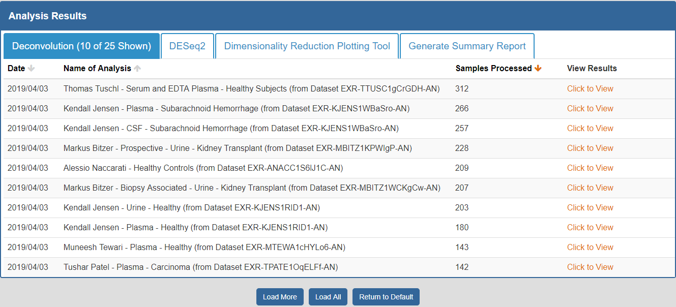
- The Date column will tell you when the analysis was run.
- The Analysis Name column will tell you the name of the analysis.
- The Samples Processed column will tell you how many samples were involved in the analysis.
- The View Results column will allow you to view the results associated with a given analysis.
- The Load More / Load All buttons will display additional results associated with a given tool (if available).
You can see an example of the public analysis results page below:
To better understand the output for a given tool, please see the "Understanding Your DESeq2 Results", "Understanding Your Dimensionality Reduction Plotting Tool Results", and "Understanding Your Generate Summary Report Results" sections below.
Running Your Own Analyses
Step 1: Selecting Your Samples of Interest
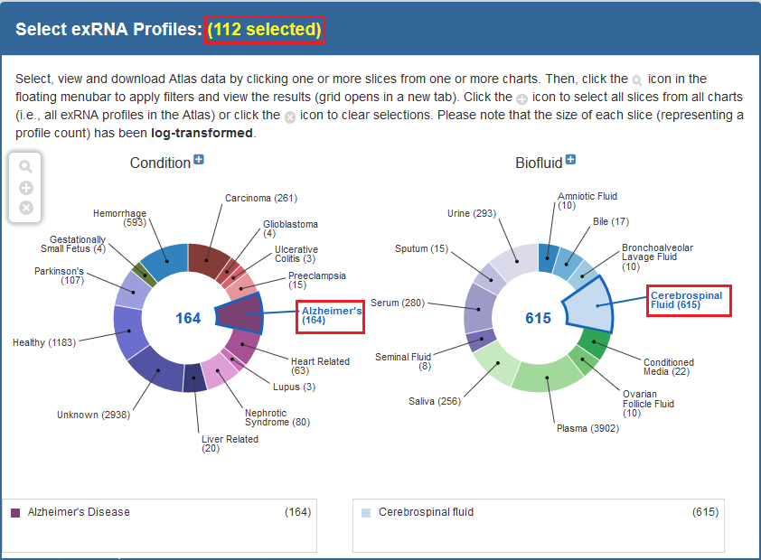
The first step to running an analysis is selecting your samples of interest.We recommend using the faceted charts or selecting a dataset from the Datasets page to select your samples (all tools may not be available for other types of grids).
- If using the faceted charts, click the appropriate facets and then click the magnifying glass icon to show corresponding samples in a grid.
- If using the Datasets page, you can click the sample count badge in the lower right corner of a given dataset card to show corresponding samples in a grid.
Below, you can see an example of how one would select samples via the faceted charts:
And here is an example of how one would select a set of samples via the Datasets page:

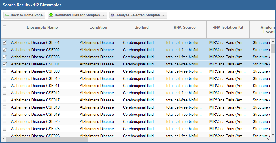
- You can select specific samples by using the checkboxes to the left of each sample.
- To select all samples, click the checkbox in the upper left corner of the grid.
- The different metadata columns (Condition, Anatomical Location, etc.) should help you figure out which specific samples you want to analyze.
- You can also click on the right side of a given column to sort that column, place filters on that column, or disable any column in the grid.
Below, you can see an example where I've selected 4 samples in my samples grid:
Step 2: Selecting and Running a Analysis Tool
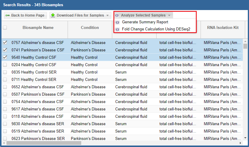
After you've selected your samples, you'll need to pick out a tool to run on those samples.You can click the "Analyze Selected Samples" button to see available tools.
- You can read more about the individual tools in the Overview of Tools section above.
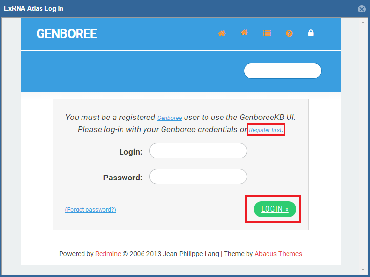
- A Genboree account is required to use the analysis tools.
- If you have an account already, just fill in your login information and then click the "Login" button.
- If you don't have an account, you can click the "Register here!" link to create one.
- Once you've logged in once, you won't need to log in again for that Atlas session.
- First, you'll need to select a Group and Database in which to store your output files.
Each Genboree account starts with a Group (named after your username), and we will offer to create a Database for you (named "Exrna-atlas Output") if you don't have one. - Next, you'll need to provide an Analysis Name for your analysis run - this name will be used to organize your analysis results, so picking an informative name is a good idea!
- Finally, some tools will require additional settings - for example, DESeq2 will require you to put in a factor name and two factor levels of interest.
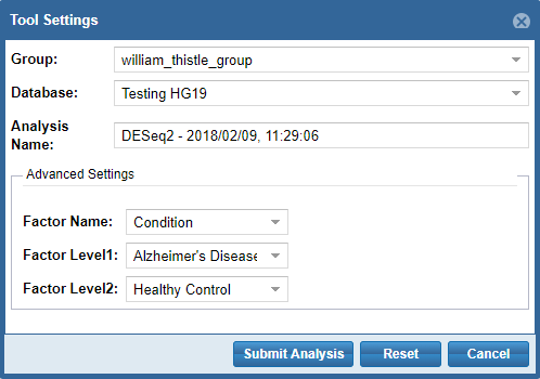
When you're ready to submit your analysis, click the Submit Analysis button.
After a moment, you will be provided an analysis job ID. You will receive an email when your analysis run is complete.
Step 3: Viewing Your Analysis Results
To view your analysis results, you can click the Analysis Results button in the Atlas navigation bar and then click the My Analysis Results button.
You will then be taken to a page where you can click between different tabs, each corresponding to a different tool.
- The Date column will tell you when the analysis was run.
- The Analysis Name column will tell you the name of the analysis.
- The Samples Processed column will tell you how many samples were involved in the analysis.
- The View Results column will allow you to view the results associated with a given analysis.
- The Load More / Load All buttons (if available) will display additional results associated with a given tool.
You can see an example of an analysis results page below:
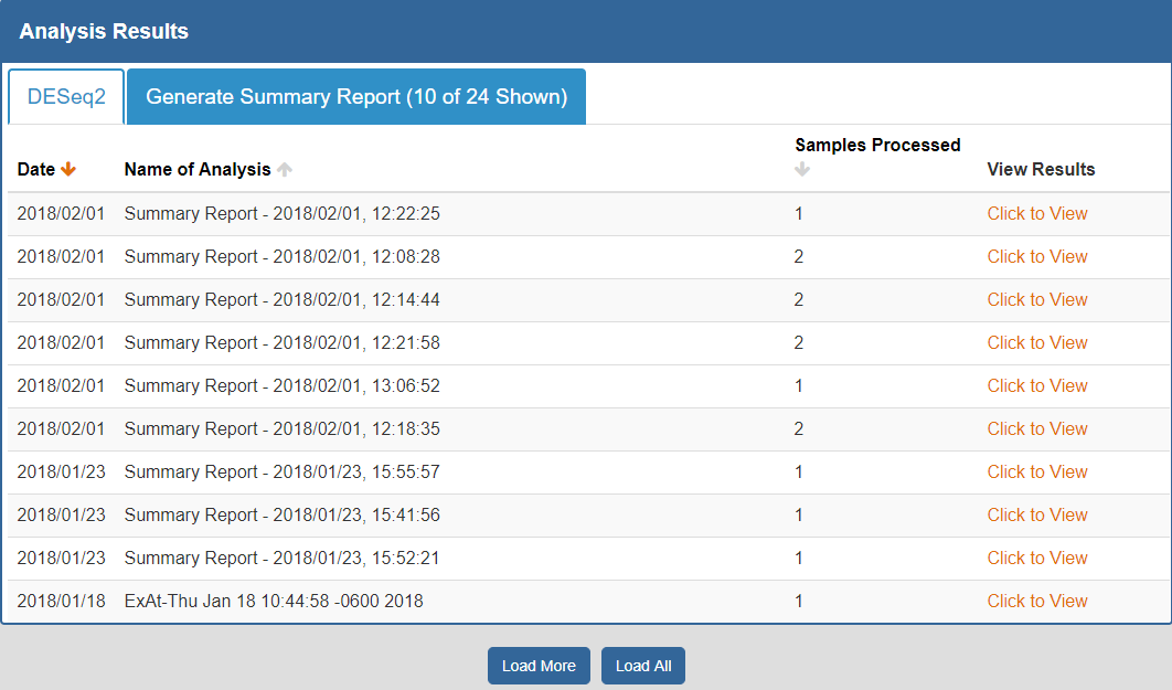
To better understand the output for a given tool, please see the "Understanding Your DESeq2 Results" and "Understanding Your Generate Summary Report Results" sections below.
Understanding Your Results
Understanding Your XDec Results
Output from XDec includes:- Stage 1 Deconvolution
- Heatmap representing the correlation between the deconvoluted cargo profiles modeled for the current dataset and the cargo types (CT) estimated from the deconvolution of individual Atlas datasets across informative ncRNAs.
- Table of estimated constituent cargo profiles across 20,000+ ncRNA [miRNA, piRNA, tRNA, Y RNA, lincRNA, snoRNA, snRNA] transcripts (expression is normalized to [0:1] range).
- Heatmap representing the proportions of each cargo profile for each sample in the current dataset.
- Table of estimated proportions of each cargo profile for each sample in the current dataset.
- Boxplots representing the proportions of each cargo profile for each sample in the current dataset separated based on provided metadata features.
- Stage 2 Deconvolution
- Tables of estimated average cargo profiles across 20,000+ ncRNA (miRNA, piRNA, tRNA, Y RNA, lincRNA, snoRNA, and snRNA) transcripts in reads per million (RPM) separated based on provided metadata features. Tables include mean expression, std. errors, degrees of freedom, and per sample residuals.
To learn more about XDec and how to interpret your results, read the Cell paper "ExRNA Atlas Analysis Reveals Distinct Extracellular RNA Cargo Types and Their Carriers Present Across Human Biofluids" (Murillo et al., 2019).
Understanding Your DESeq2 Results
When you click to view your DESeq2 results, a new page will open up containing differentially expressed miRNAs for the selected Atlas data.Each row corresponds to a given miRNA, and each column is explained below:
- The Checkbox column allows you to select miRNAs for further downstream analysis.
- You can click the checkbox next to a given miRNA (highlighted in blue below) to select that miRNA.
- You can click the checkbox in the upper left corner of the table (highlighted in green below) to select all visible miRNAs.
- The Identifiers column contains all of your miRNA identifiers.
- The Base Mean column contains "the average of the normalized count values, divided by the size factors, taken over all samples [in the original dataset]" for each miRNA. [1]
- The log2 Fold Change column contains the "effect size estimate" for each miRNA. [1]
- The Standard Error column contains the "standard error estimate for the log2 fold change estimate" for each miRNA. [1]
- The p-value column contains the Wald test p-value for each miRNA. [1]
- The Adjusted p-value column contains the Benjamini-Hochberg adjusted p-value for each miRNA. [1]
[1] Love, M. I., Anders, S., Kim V., & Huber W. (2017, Aug 9). RNA-seq workflow: gene-level exploratory analysis and differential expression.
Retrieved from http://www.bioconductor.org/help/workflows/rnaseqGene/
By default, the table is sorted by adjusted p-value, but you can sort by any of the columns.
In addition, you can perform downstream analysis on selected miRNAs of interest by clicking the Analyze Selected miRNAs button (highlighted in red below) above the table.
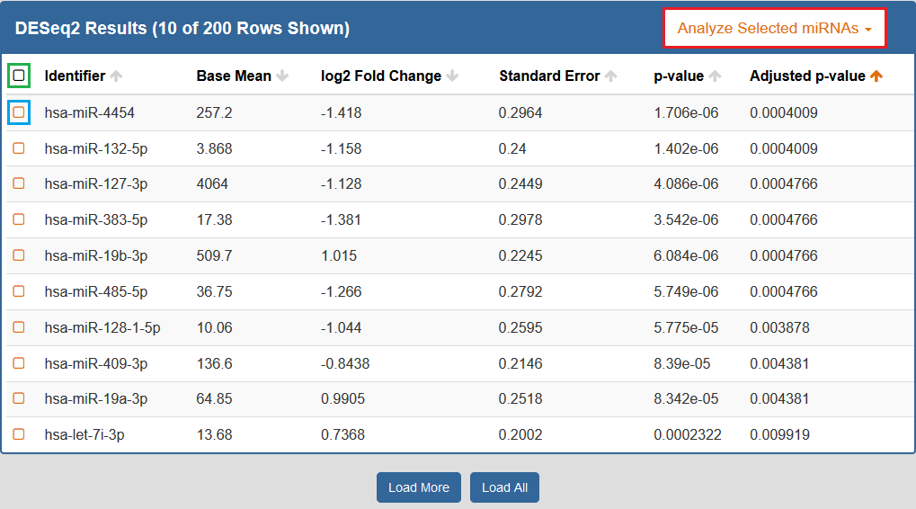
See descriptions of all available downstream analysis tools below.
Pathway Finder
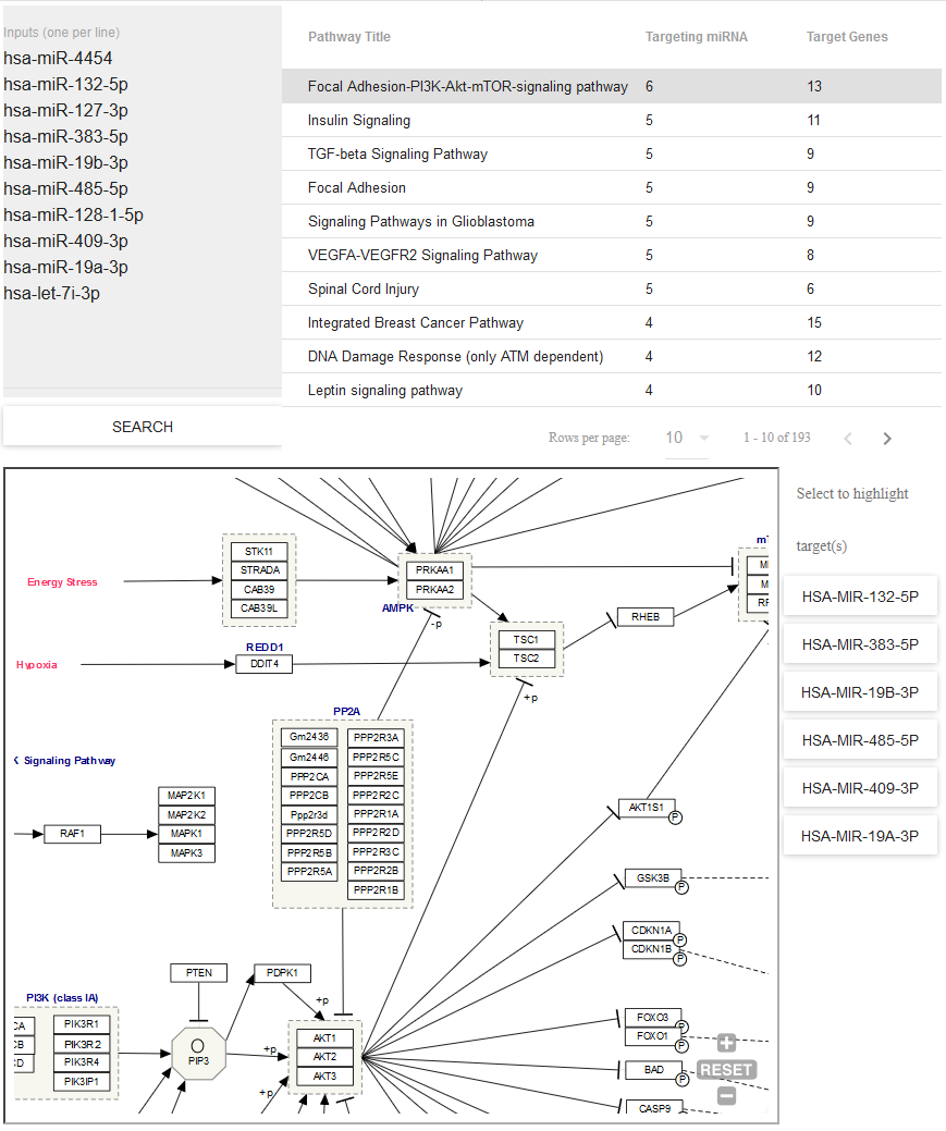
- Use Pathway Finder (hosted by WikiPathways) to find pathways containing miRNAs of interest (or protein targets of those miRNAs).
- Click a given pathway title to visualize its contents at the bottom of the page.
- Then, select a given miRNA to highlight its associated target(s).
- The pathway visualization is interactive - zoom in or out by using the + and - icons, and click a given gene product to learn more about it.
- Designed and implemented by Kristina Hanspers, Anders Riutta, and Alexander Pico at the Gladstone Institutes, San Francisco, CA.
- Integrated into the exRNA Atlas by William Thistlethwaite and Neethu Shah at the Bioinformatics Research Lab, Baylor College of Medicine, Houston, TX.
You can see what the Pathway Finder interface looks like below:
Understanding Your Dimensionality Reduction Plotting Tool Results
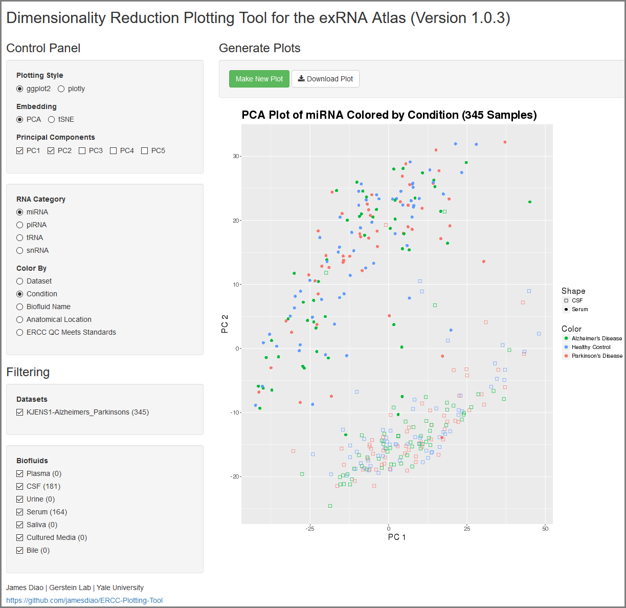
When you click to view your Dimensionality Reduction Plotting Tool results, a new page will open up containing an interface for visualizing the expression of different ncRNAs in the selected Atlas data.
On the left side of the screen, you will see the Control Panel and Filtering Panel that allow you to configure your visualization.
- The Plotting Style setting allows you to choose between two different plotting tools (ggplot2 and plotly).
- Note that ggplot2 supports 2D plots while plotly supports both 2D and 3D plots.
- The Embedding setting allows you to choose between PCA and tSNE embedding.
- If you currently have PCA selected, you can choose between the top 5 principal components using the Principal Components setting.
- The RNA Category setting allows you to choose the type of ncRNA you'd like to plot.
- The Color By setting allows you to choose how you'd like to color your plot.
- The Datasets setting allows you to to add or remove different datasets from your plot (with dynamically adjusted counts for each option).
- Note that these filters are purely visual and do not recompute the PCA or tSNE values.
- The Biofluids setting allows you to to add or remove different biofluids from your plot (with dynamically adjusted counts for each option).
- Note that these filters are purely visual and do not recompute the PCA or tSNE values.
After you've selected your settings, you can click the Make New Plot button on the right side of the screen to generate a new visualization based on your current Control Panel and Filtering Panel settings.
You can then download a PDF of your current visualization by clicking the Download Plot button.
Understanding Your Generate Summary Report Results
When you click to view your Generate Summary Report results, you will download an archive containing a variety of summary files describing the selected Atlas data.
Descriptions of the summary files can be found below:
| File Name | Description of File |
| QC Data | |
| [analysisName]_exceRpt_DiagnosticPlots.pdf | All diagnostic plots automatically generated by the tool |
| [analysisName]_exceRpt_readMappingSummary.txt | Read-alignment summary including total counts for each library |
| [analysisName]_exceRpt_ReadLengths.txt | Read-lengths (after 3' adapters/barcodes are removed) |
| [analysisName]_exceRpt_QCresults.txt | QC statistics for all samples |
| Raw Transcriptome Quantifications | |
| [analysisName]_exceRpt_miRNA_ReadCounts.txt | miRNA read-counts quantifications |
| [analysisName]_exceRpt_tRNA_ReadCounts.txt | tRNA read-counts quantifications |
| [analysisName]_exceRpt_piRNA_ReadCounts.txt | piRNA read-counts quantifications |
| [analysisName]_exceRpt_gencode_ReadCounts.txt | gencode read-counts quantifications |
| [analysisName]_exceRpt_circularRNA_ReadCounts.txt | circularRNA read-count quantifications |
| [analysisName]_exceRpt_biotypeCounts.txt | biotype read-count quantifications |
| [analysisName]_exceRpt_exogenous_miRNA_ReadCounts.txt | exogenous miRNA read-counts quantifications |
| Normalized Transcriptome Quantifications | |
| [analysisName]_exceRpt_miRNA_ReadsPerMillion.txt | miRNA RPM quantifications |
| [analysisName]_exceRpt_tRNA_ReadsPerMillion.txt | tRNA RPM quantifications |
| [analysisName]_exceRpt_piRNA_ReadsPerMillion.txt | piRNA RPM quantifications |
| [analysisName]_exceRpt_gencode_ReadsPerMillion.txt | gencode RPM quantifications |
| [analysisName]_exceRpt_circularRNA_ReadsPerMillion.txt | circularRNA RPM quantifications |
| [analysisName]_exceRpt_exogenous_miRNA_ReadsPerMillion.txt | exogenous miRNA RPM quantifications |
| Exogenous Genomic Taxonomies | |
| [analysisName]_exceRpt_exogenousGenomes_taxonomyCumulative_ReadCounts.txt | cumulative taxonomy read-count quantifications |
| [analysisName]_exceRpt_exogenousGenomes_taxonomyCumulative_ReadsPerMillion.txt | cumulative taxonomy RPM quantifications |
| [analysisName]_exceRpt_exogenousGenomes_taxonomySpecific_ReadCounts.txt | specific taxonomy read-count quantifications |
| [analysisName]_exceRpt_exogenousGenomes_taxonomySpecific_ReadsPerMillion.txt | specific taxonomy RPM quantifications |
| [analysisName]_exceRpt_exogenousGenomes_TaxonomyTrees_aggregateSamples.pdf | visualized taxonomy tree for samples, aggregated |
| [analysisName]_exceRpt_exogenousGenomes_TaxonomyTrees_perSample.pdf | visualized taxonomy trees for each sample |
| Exogenous rRNA Taxonomies | |
| [analysisName]_exceRpt_exogenousRibosomal_taxonomyCumulative_ReadCounts.txt | cumulative taxonomy read-count quantifications |
| [analysisName]_exceRpt_exogenousRibosomal_taxonomyCumulative_ReadsPerMillion.txt | cumulative taxonomy RPM quantifications |
| [analysisName]_exceRpt_exogenousRibosomal_taxonomySpecific_ReadCounts.txt | specific taxonomy read-count quantifications |
| [analysisName]_exceRpt_exogenousRibosomal_taxonomySpecific_ReadsPerMillion.txt | specific taxonomy RPM quantifications |
| [analysisName]_exceRpt_exogenousRibosomal_TaxonomyTrees_aggregateSamples.pdf | visualized taxonomy tree for samples, aggregated |
| [analysisName]_exceRpt_exogenousRibosomal_TaxonomyTrees_perSample.pdf | visualized taxonomy trees for each sample |
| R Objects | |
| [analysisName]_exceRpt_smallRNAQuants_ReadCounts.RData | All raw data (binary R object) |
| [analysisName]_exceRpt_smallRNAQuants_ReadsPerMillion.RData | All normalized data (binary R object) |
| Other | |
| [analysisName]_exceRpt_sampleGroupDefinitions.txt | Information about sample groups (not used by Atlas) |
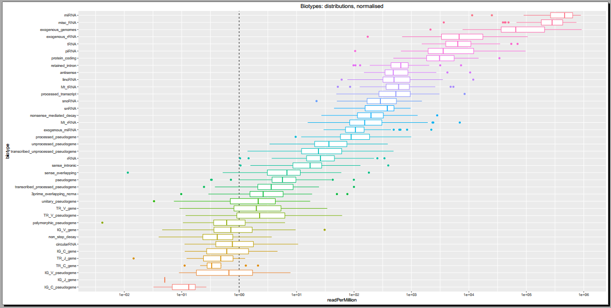
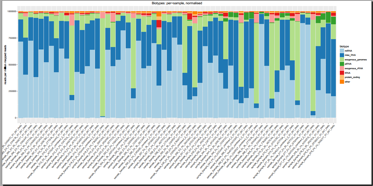
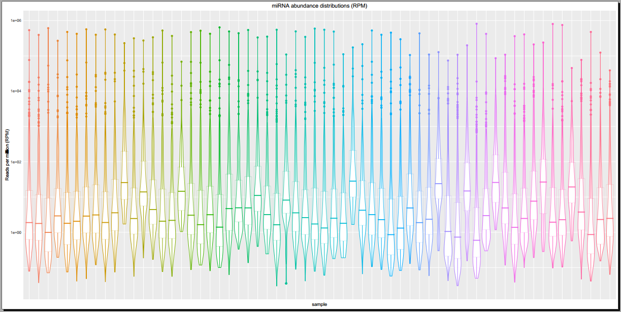
Below, you can see some example plots from the Diagnostic Plots PDF referenced above.
