Index by title
Batch Download of Atlas Files
Coming soon!
Overview
Introduction
The exRNA Atlas contains a number of different analysis tools for analyzing Atlas RNA-seq data:
- DESeq2, a differential expression analysis tool
- Dimensionality Reduction Plotting Tool, a visualization tool that allows users to see miRNA expression via PCA and tSNE embedding.
- Generate Summary Report, a tool which summarizes output from multiple samples processed through exceRpt into one cohesive report
Below, we will demonstrate how to use these tools on Atlas data and see your analysis results in the Atlas.
Before we begin describing how to use the analysis tools, we'll go over what each tool does in more detail.
Currently, all analysis tools work solely with RNA-seq profiles.
DESeq2
- View a table containing differentially expressed miRNAs for selected Atlas data.
- Sort data by a variety of different metrics (adjusted p-value by default).
- Select some subset of miRNAs and use the Pathway Finder tool to find pathways containing miRNAs of interest (or protein targets of those miRNAs).
- Currently, our integration of the tool allows for pairwise comparisons of sample profiles (two conditions, two RNA isolation kits, etc.).
- Tool designed and implemented by Michael Love, Simon Anders, and Wolfgang Huber (PubMed).
- Integrated into the exRNA Atlas by William Thistlethwaite and Neethu Shah at the Bioinformatics Research Lab, Baylor College of Medicine, Houston, TX.
Dimensionality Reduction Plotting Tool
- Visualize selected Atlas data via PCA and tSNE embedding.
- Choose between three different plotting styles (ggplot2, plotly 2D, and plotly 3D).
- Pick between four different RNA categories (miRNA, piRNA, tRNA, snRNA) for your visualization.
- Color your plots by various metadata categories like dataset, anatomical location, condition, and biofluid name.
- Use filters to add or remove different datasets and biofluids from a given plot (with dynamically adjusted counts for each option).
- Note that these filters are purely visual and do not recompute the PCA or tSNE values.
- Currently, only precomputed analyses are available for this tool.
- Tool designed and implemented by James Diao and Joel Rozowsky at the Gerstein Lab, Yale University, New Haven, CT.
- Integrated into the exRNA Atlas by William Thistlethwaite and Andrew R. Jackson at the Bioinformatics Research Lab, Baylor College of Medicine, Houston, TX.
Generate Summary Report
- Download an archive containing a collection of summary files describing the output from exceRpt for selected samples.
- Summary files include:
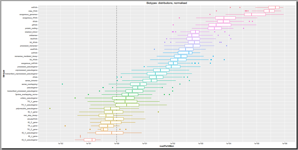
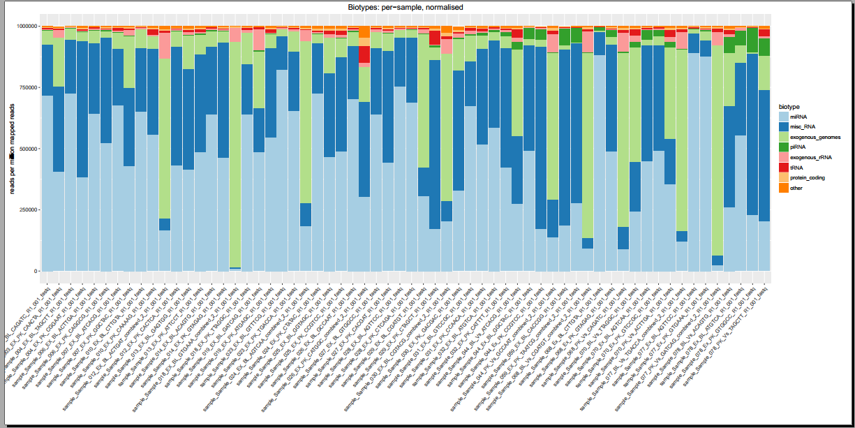
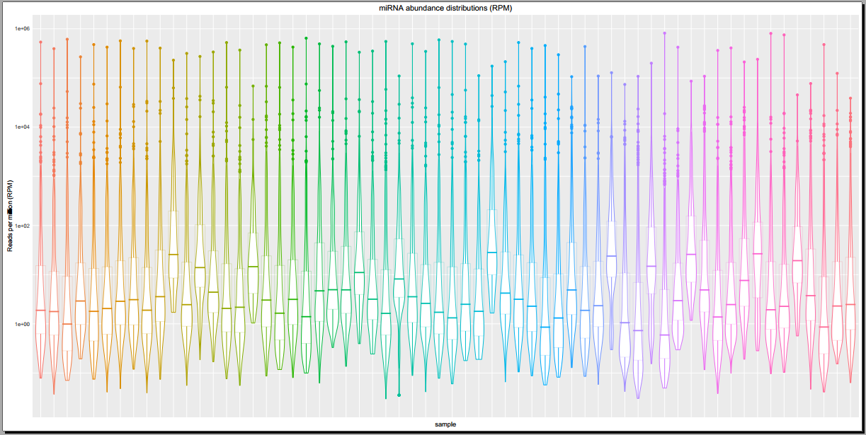
- Plots including read count distributions, biotype distributions, miRNA abundance distributions, etc.
- Read count tables for each library (miRNA / tRNA / piRNA / etc.) that span all selected samples. Both raw counts and normalized counts (reads per million mapped reads) are available.
- Visualized taxonomy trees for exogenous rRNA and exogenous genomic reads.
- A full list of summary files can be found on the exceRpt Tutorial Page.
- Tool designed and implemented by Rob Kitchen and Joel Rozowsky at the Gerstein Lab, Yale University, New Haven, CT.
- Integrated into the exRNA Atlas by William Thistlethwaite and Neethu Shah at the Bioinformatics Research Lab, Baylor College of Medicine, Houston, TX.
Viewing Public Analysis Results
Before running your own analyses, you may be interested in viewing the Atlas' public analysis results.
- These results are available to everyone and cover much of the Atlas data.
- They should be useful for an initial examination of what the Atlas has to offer.
To view the Atlas' public analysis results, you can click the Analysis Results button in the Atlas navigation bar and then click the Public Analysis Results button.
You will then be taken to a page where you can click between different tabs, each corresponding to a different tool.
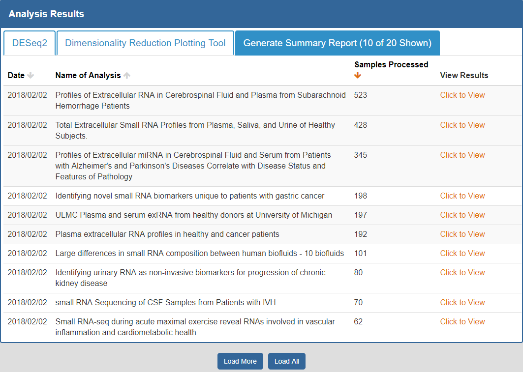
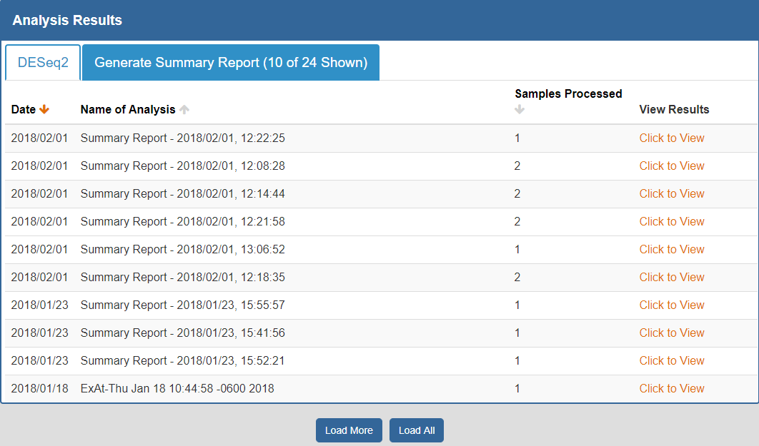
When you click a given tab, you will see the public analysis results associated with that tool:
- The Date column will tell you when the analysis was run.
- The Analysis Name column will tell you the name of the analysis.
- The Samples Processed column will tell you how many samples were involved in the analysis.
- The View Results column will allow you to view the results associated with a given analysis.
- The Load More / Load All buttons will display additional results associated with a given tool (if available).
You can see an example of the public analysis results page below:
To better understand the output for a given tool, please see the "Understanding Your DESeq2 Results", "Understanding Your Dimensionality Reduction Plotting Tool Results", and "Understanding Your Generate Summary Report Results" sections below.
Running Your Own Analyses
Step 1: Selecting Your Samples of Interest
The first step to running an analysis is selecting your samples of interest.
We recommend using the faceted charts or selecting a dataset from the Datasets page to select your samples (all tools may not be available for other types of grids).
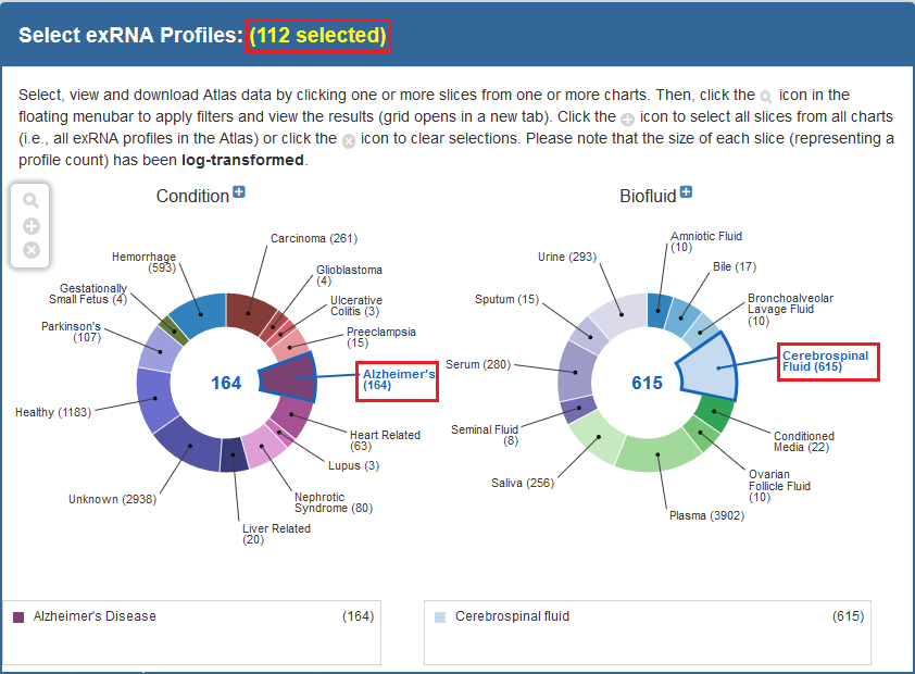
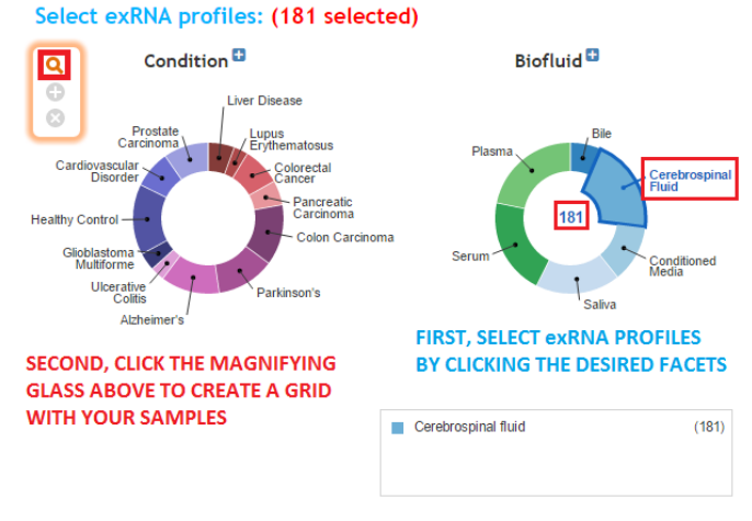
- If using the faceted charts, click the appropriate facets and then click the magnifying glass icon to show corresponding samples in a grid.
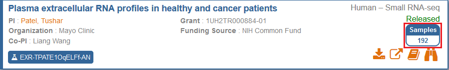
- If using the Datasets page, you can click the sample count badge in the lower right corner of a given dataset card to show corresponding samples in a grid.
Below, you can see an example of how one would select samples via the faceted charts:
And here is an example of how one would select a set of samples via the Datasets page:
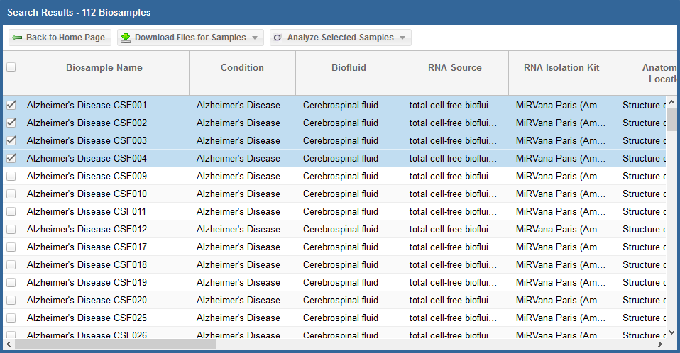
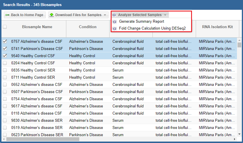
After you have generated your grid, you will need to select the specific samples you want to analyze.
- You can select specific samples by using the checkboxes to the left of each sample.
- To select all samples, click the checkbox in the upper left corner of the grid.
- The different metadata columns (Condition, Anatomical Location, etc.) should help you figure out which specific samples you want to analyze.
- You can also click on the right side of a given column to sort that column, place filters on that column, or disable any column in the grid.
Below, you can see an example where I've selected 4 samples in my samples grid:
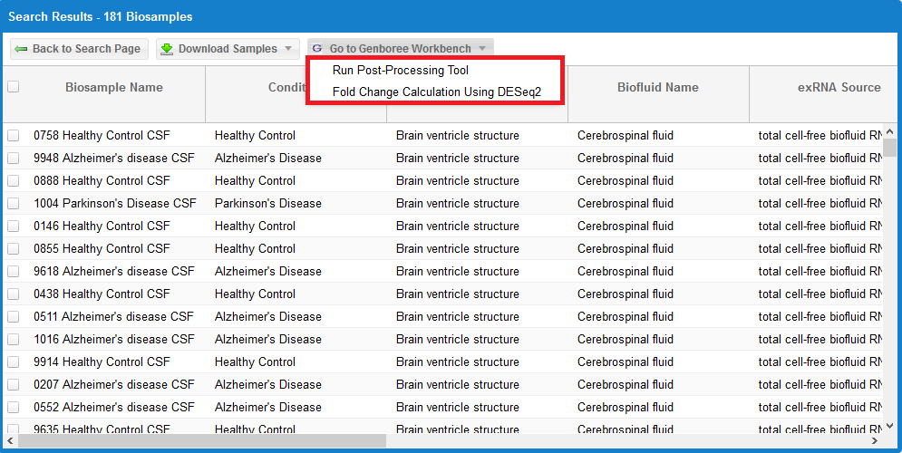
After you've selected your samples, you'll need to pick out a tool to run on those samples.
You can click the "Analyze Selected Samples" button to see available tools.
- You can read more about the individual tools in the Overview of Tools section above.
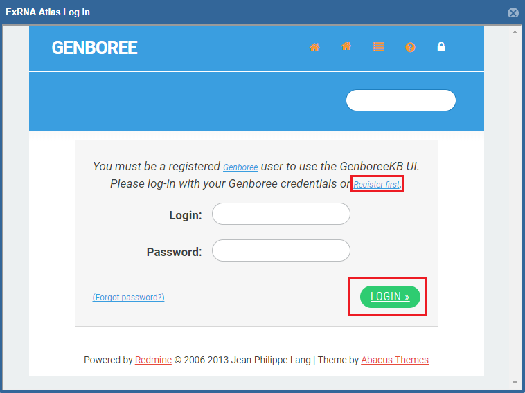
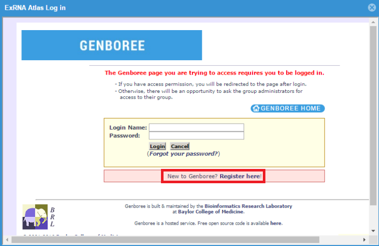
After choosing a tool, you will be prompted to log into your Genboree account (unless you are already logged in).
- A Genboree account is required to use the analysis tools.
- If you have an account already, just fill in your login information and then click the "Login" button.
- If you don't have an account, you can click the "Register here!" link to create one.
- Once you've logged in once, you won't need to log in again for that Atlas session.
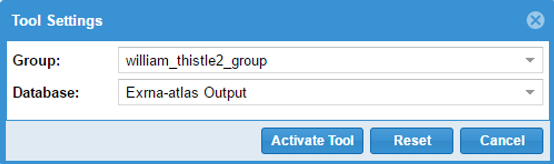
After you've logged in, you'll be prompted to provide settings for your analysis run.
- First, you'll need to select a Group and Database in which to store your output files.
Each Genboree account starts with a Group (named after your username), and we will offer to create a Database for you (named "Exrna-atlas Output") if you don't have one.
- Next, you'll need to provide an Analysis Name for your analysis run - this name will be used to organize your analysis results, so picking an informative name is a good idea!
- Finally, some tools will require additional settings - for example, DESeq2 will require you to put in a factor name and two factor levels of interest.
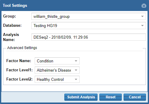
When you're ready to submit your analysis, click the Submit Analysis button.
After a moment, you will be provided an analysis job ID. You will receive an email when your analysis run is complete.
Step 3: Viewing Your Analysis Results
To view your analysis results, you can click the Analysis Results button in the Atlas navigation bar and then click the My Analysis Results button.
You will then be taken to a page where you can click between different tabs, each corresponding to a different tool.
When you click a given tab, you will see any analysis results associated with that tool:
- The Date column will tell you when the analysis was run.
- The Analysis Name column will tell you the name of the analysis.
- The Samples Processed column will tell you how many samples were involved in the analysis.
- The View Results column will allow you to view the results associated with a given analysis.
- The Load More / Load All buttons (if available) will display additional results associated with a given tool.
You can see an example of an analysis results page below:
To better understand the output for a given tool, please see the "Understanding Your DESeq2 Results", "Understanding Your Dimensionality Reduction Plotting Tool Results", and "Understanding Your Generate Summary Report Results" sections below.
Understanding Your Results
Understanding Your DESeq2 Results
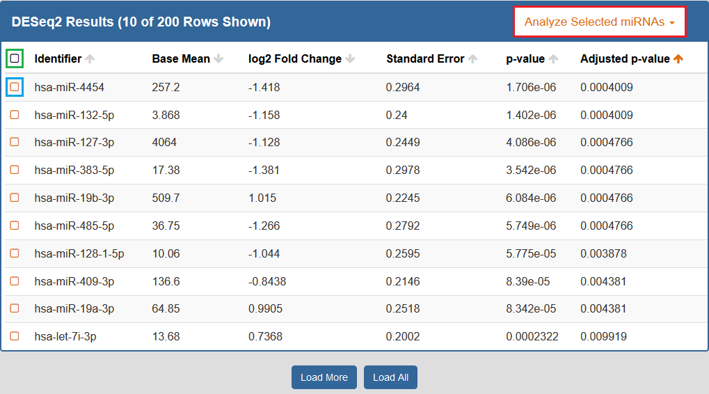
When you click to view your DESeq2 results, a new page will open up containing differentially expressed miRNAs for the selected Atlas data.
Each row corresponds to a given miRNA, and each column is explained below:
- The Checkbox column allows you to select miRNAs for further downstream analysis.
- You can click the checkbox next to a given miRNA (highlighted in blue below) to select that miRNA.
- You can click the checkbox in the upper left corner of the table (highlighted in green below) to select all visible miRNAs.
- The Identifiers column contains all of your miRNA identifiers.
- The Base Mean column contains "the average of the normalized count values, divided by the size factors, taken over all samples [in the original dataset]" for each miRNA. [1]
- The log2 Fold Change column contains the "effect size estimate" for each miRNA. [1]
- The Standard Error column contains the "standard error estimate for the log2 fold change estimate" for each miRNA. [1]
- The p-value column contains the Wald test p-value for each miRNA. [1]
- The Adjusted p-value column contains the Benjamini-Hochberg adjusted p-value for each miRNA. [1]
[1] Love, M. I., Anders, S., Kim V., & Huber W. (2017, Aug 9). RNA-seq workflow: gene-level exploratory analysis and differential expression.
Retrieved from http://www.bioconductor.org/help/workflows/rnaseqGene/
By default, the table is sorted by adjusted p-value, but you can sort by any of the columns.
In addition, you can perform downstream analysis on selected miRNAs of interest by clicking the Analyze Selected miRNAs button (highlighted in red below) above the table.
See descriptions of all available downstream analysis tools below.
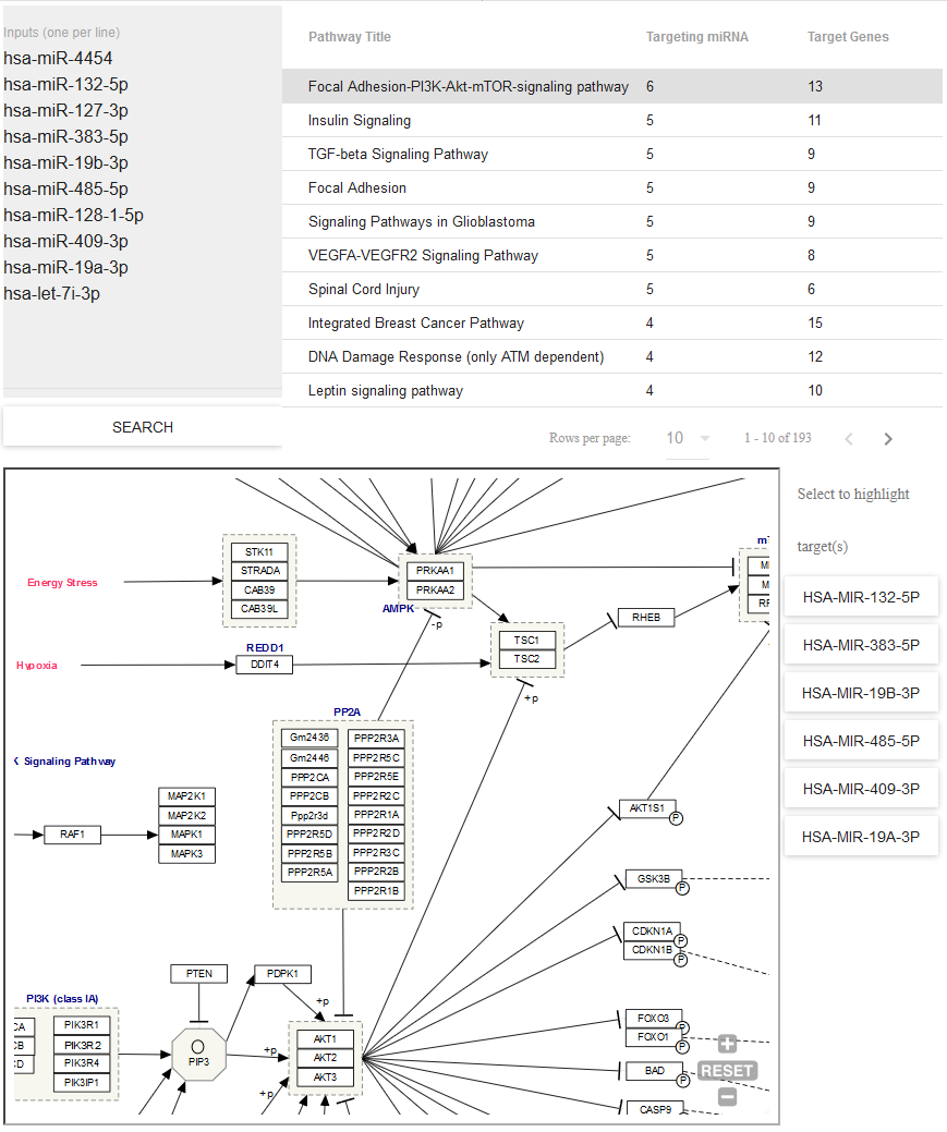
Pathway Finder
- Use Pathway Finder (hosted by WikiPathways) to find pathways containing miRNAs of interest (or protein targets of those miRNAs).
- Click a given pathway title to visualize its contents at the bottom of the page.
- Then, select a given miRNA to highlight its associated target(s).
- The pathway visualization is interactive - zoom in or out by using the + and - icons, and click a given gene product to learn more about it.
- Designed and implemented by Kristina Hanspers, Anders Riutta, and Alexander Pico at the Gladstone Institutes, San Francisco, CA.
- Integrated into the exRNA Atlas by William Thistlethwaite and Neethu Shah at the Bioinformatics Research Lab, Baylor College of Medicine, Houston, TX.
You can see what the Pathway Finder interface looks like below:
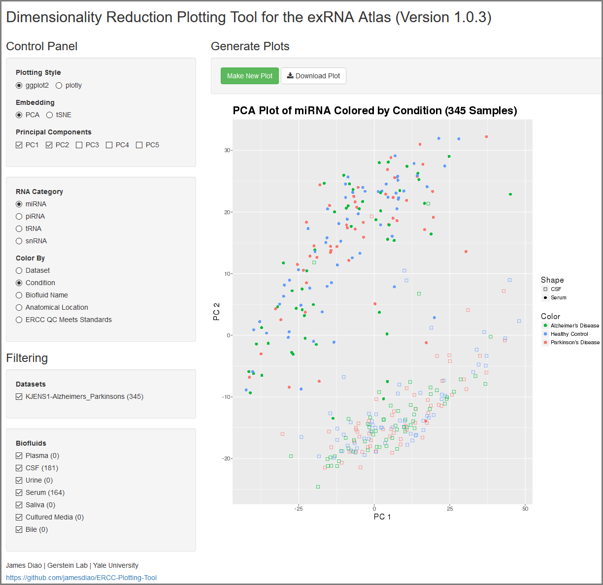
When you click to view your Dimensionality Reduction Plotting Tool results, a new page will open up containing an interface for visualizing the expression of different ncRNAs in the selected Atlas data.
On the left side of the screen, you will see the Control Panel and Filtering Panel that allow you to configure your visualization.
Within the Control Panel, you will see the following settings:
- The Plotting Style setting allows you to choose between two different plotting tools (ggplot2 and plotly).
- Note that ggplot2 supports 2D plots while plotly supports both 2D and 3D plots.
- The Embedding setting allows you to choose between PCA and tSNE embedding.
- If you currently have PCA selected, you can choose between the top 5 principal components using the Principal Components setting.
- The RNA Category setting allows you to choose the type of ncRNA you'd like to plot.
- The Color By setting allows you to choose how you'd like to color your plot.
Within the Filtering Panel, you will see the following settings:
- The Datasets setting allows you to to add or remove different datasets from your plot (with dynamically adjusted counts for each option).
- Note that these filters are purely visual and do not recompute the PCA or tSNE values.
- The Biofluids setting allows you to to add or remove different biofluids from your plot (with dynamically adjusted counts for each option).
- Note that these filters are purely visual and do not recompute the PCA or tSNE values.
After you've selected your settings, you can click the Make New Plot button on the right side of the screen to generate a new visualization based on your current Control Panel and Filtering Panel settings.
You can then download a PDF of your current visualization by clicking the Download Plot button.
Understanding Your Generate Summary Report Results
When you click to view your Generate Summary Report results, you will download an archive containing a variety of summary files describing the selected Atlas data.
Descriptions of the summary files can be found below:
| File Name |
Description of File |
| QC Data |
|
| [analysisName]_exceRpt_DiagnosticPlots.pdf |
All diagnostic plots automatically generated by the tool |
| [analysisName]_exceRpt_readMappingSummary.txt |
Read-alignment summary including total counts for each library |
| [analysisName]_exceRpt_ReadLengths.txt |
Read-lengths (after 3' adapters/barcodes are removed) |
| [analysisName]_exceRpt_QCresults.txt |
QC statistics for all samples |
| Raw Transcriptome Quantifications |
|
| [analysisName]_exceRpt_miRNA_ReadCounts.txt |
miRNA read-counts quantifications |
| [analysisName]_exceRpt_tRNA_ReadCounts.txt |
tRNA read-counts quantifications |
| [analysisName]_exceRpt_piRNA_ReadCounts.txt |
piRNA read-counts quantifications |
| [analysisName]_exceRpt_gencode_ReadCounts.txt |
gencode read-counts quantifications |
| [analysisName]_exceRpt_circularRNA_ReadCounts.txt |
circularRNA read-count quantifications |
| [analysisName]_exceRpt_biotypeCounts.txt |
biotype read-count quantifications |
| [analysisName]_exceRpt_exogenous_miRNA_ReadCounts.txt |
exogenous miRNA read-counts quantifications |
| Normalized Transcriptome Quantifications |
|
| [analysisName]_exceRpt_miRNA_ReadsPerMillion.txt |
miRNA RPM quantifications |
| [analysisName]_exceRpt_tRNA_ReadsPerMillion.txt |
tRNA RPM quantifications |
| [analysisName]_exceRpt_piRNA_ReadsPerMillion.txt |
piRNA RPM quantifications |
| [analysisName]_exceRpt_gencode_ReadsPerMillion.txt |
gencode RPM quantifications |
| [analysisName]_exceRpt_circularRNA_ReadsPerMillion.txt |
circularRNA RPM quantifications |
| [analysisName]_exceRpt_exogenous_miRNA_ReadsPerMillion.txt |
exogenous miRNA RPM quantifications |
| Exogenous Genomic Taxonomies |
|
| [analysisName]_exceRpt_exogenousGenomes_taxonomyCumulative_ReadCounts.txt |
cumulative taxonomy read-count quantifications |
| [analysisName]_exceRpt_exogenousGenomes_taxonomyCumulative_ReadsPerMillion.txt |
cumulative taxonomy RPM quantifications |
| [analysisName]_exceRpt_exogenousGenomes_taxonomySpecific_ReadCounts.txt |
specific taxonomy read-count quantifications |
| [analysisName]_exceRpt_exogenousGenomes_taxonomySpecific_ReadsPerMillion.txt |
specific taxonomy RPM quantifications |
| [analysisName]_exceRpt_exogenousGenomes_TaxonomyTrees_aggregateSamples.pdf |
visualized taxonomy tree for samples, aggregated |
| [analysisName]_exceRpt_exogenousGenomes_TaxonomyTrees_perSample.pdf |
visualized taxonomy trees for each sample |
| Exogenous rRNA Taxonomies |
|
| [analysisName]_exceRpt_exogenousRibosomal_taxonomyCumulative_ReadCounts.txt |
cumulative taxonomy read-count quantifications |
| [analysisName]_exceRpt_exogenousRibosomal_taxonomyCumulative_ReadsPerMillion.txt |
cumulative taxonomy RPM quantifications |
| [analysisName]_exceRpt_exogenousRibosomal_taxonomySpecific_ReadCounts.txt |
specific taxonomy read-count quantifications |
| [analysisName]_exceRpt_exogenousRibosomal_taxonomySpecific_ReadsPerMillion.txt |
specific taxonomy RPM quantifications |
| [analysisName]_exceRpt_exogenousRibosomal_TaxonomyTrees_aggregateSamples.pdf |
visualized taxonomy tree for samples, aggregated |
| [analysisName]_exceRpt_exogenousRibosomal_TaxonomyTrees_perSample.pdf |
visualized taxonomy trees for each sample |
| R Objects |
|
| [analysisName]_exceRpt_smallRNAQuants_ReadCounts.RData |
All raw data (binary R object) |
| [analysisName]_exceRpt_smallRNAQuants_ReadsPerMillion.RData |
All normalized data (binary R object) |
| Other |
|
| [analysisName]_exceRpt_sampleGroupDefinitions.txt |
Information about sample groups (not used by Atlas) |
Below, you can see some example plots from the Diagnostic Plots PDF referenced above.
Overview
Comparative and Downstream Analysis of Samples Using the Genboree Workbench
- We have a number of different downstream / comparative analysis tools available in the exRNA Atlas.
- By selecting your samples of interest and then selecting your tool of interest, you can move into the Genboree Workbench where you can then perform your analysis.
- We will go through the process step-by-step below.
Step 1: Selecting Your Samples of Interest
- The first step to running your analysis is selecting your samples of interest.
- We recommend using the faceted charts (all tools may not be available for other types of grids).
- Click the appropriate facets and then click the magnifying glass icon to show corresponding samples in a grid.
- After you have generated your grid, you will need to select the specific samples you want to analyze.
- You can select specific samples by using the checkboxes to the left of each sample.
- To select all samples, click the checkbox in the upper left corner of the grid.
- The different metadata columns (Condition, Anatomical Location, etc.) should help you figure out which specific samples you want to analyze.
- You can also click on the right side of a given column to sort that column, place filters on that column, or disable any column in the grid.
- After you've selected your samples, you'll need to pick out a tool to run on those samples.
- You can click the "Go to Genboree Workbench" button to see available tools.
- We currently have the following tools available:
- You will be prompted to log into the Genboree Workbench once you choose a tool.
- This means that you must have a Genboree account in order to use the tools.
- If you have an account already, just fill in your login information and then click the "Login" button.
- If you don't have an account, you can click the "Register here!" link to create one.
- Once you've logged in once, you won't need to log in again for that Atlas session.
- After you've logged in, you'll be able to select the Group and Database which you want to use to store your output files for that tool run.
- Each Genboree account starts with a Group (named after your username), but you will need to create a Database to use the tools.
- If the Group you select doesn't already have a Database, we will offer to create a Database for you (named "Exrna-atlas Output").
- To learn more about Genboree Groups and Databases, see this FAQ page.
- Once you click "Activate Tool", you will be taken to the Genboree Workbench.
- Your Input Data panel and Output Targets panel will be filled in automatically by the Atlas.
- You can then select your tool of interest from the Workbench menu bar, fill out the appropriate settings, and then launch a tool job.
Creating an Archive
- Your submission will contain two different archives: data and metadata.
- The directions below will provide some insight on how to prepare an archive on your computer.
- IMPORTANT: If you are creating your data archive on a Mac, please create a .tar.gz and not a .zip.
We have run into some issues with decompressing large zip archives that were created using the Mac archiving software.
Using GUI-based programs
- There are plenty of GUI-based (graphical user interface) programs for compressing data.
- Below are two commonly used programs that will allow you to compress your data and metadata archives into their respective .zip files.
7-Zip will also allow you to create .tar.gz files.
Using Command Line (Terminal)
- You can also use the terminal to create your archives.
- First, open the terminal and navigate to the directory where your files are located.
- EXAMPLE: if my files are located in "C:/Users/John/Desktop/Submission", I would use the "cd" command to navigate there.
- In Windows, I would type:
cd C:/Users/John/Desktop/Submission
- In Unix/Linux/Mac OSX, I would type:
cd /home/myHome/myDir/DataFiles/
Creating a .zip Archive
- After navigating to the directory above, I would compress my files by using the "zip" command with the "-X" parameter.
- The "-X" parameter is used to avoid saving extra file attributes.
- EXAMPLE: I am creating my data archive which consists of ten different samples, each ending in the .fq.gz file extension.
- I want to name my data archive "test_data.zip".
- In order to compress my files, I would type the following::
zip -X test_data.zip *.fq.gz
- Here, *.fq.gz means that I want to include all files in my current directory that end with .fq.gz.
- I would follow a very similar process in creating my metadata archive. There are only two differences:
- I would choose a different file name ("test_metadata.zip").
- I would choose a different file extension for the end of the command (*.metadata.tsv instead of *.fq.gz).
- IMPORTANT: if you have a spike-in FASTA file in your data archive, then you would type something like the following:
zip -X test_data.zip *.fq.gz mySpikeInFile.fasta
- Here, we are archiving all .fq.gz files as well as a .fasta file named "mySpikeInFile.fasta".
Creating a .tar.gz Archive
- The directions for creating a .tar.gz archive are very similar to the directions given above for .zip files.
- The only difference is the command you use to archive your files.
- EXAMPLE: If I wanted to archive 10 different .fq.gz files as well as a spike-in FASTA file, I would type:
tar -cvzf test_data.tar.gz *.fq.gz mySpikeInFile.fasta
N/A
Creating Your FTP Account
Step 1. Create Your Genboree Account
- Before you can obtain an account on our FTP server, you will first need to create an account on Genboree:
- In order to submit your files, you will need to log into GenboreeKB once (to activate your account).
Go to GenboreeKB and log in using your Genboree username and password.
- Next, e-mail exRNA Team (coordinator for DCC at BCM) with the following information:
- Lab name
- PI name
- Genboree username(s) who will be submitting files
- The exRNA Team will create an FTP account for the listed Genboree username(s) and then email you the name of your lab's private, unique directory.
You will use this directory to submit your files.
- You will then be able to log into our FTP server (ftps://ftps.genboree.org ) using your Genboree credentials (same user name / password).
Once you log in, you will see your lab's shared directory.
Note that you will need to use an FTP client (like FileZilla) and will not be able to access your lab's directory via your web browser.
Summary
- Create an account on Genboree
- Activate your GenboreeKB account
- E-mail exRNA Team with information about your lab (lab name, PI name, Genboree user name(s) that need access)
- Wait for e-mail confirming that FTP account has been created. You can then log into our FTP server (ftp.genboree.org) using your Genboree credentials.
N/A
Common Fund exRNA Communication Consortium (ERCC) Data Sharing and Access Policy
Revised December, 2015
The ERCC. The ERCC is a community resource project designed to catalyze exRNA research activities in the scientific community. Thus, data are shared with the scientific community PRIOR to publication. In pre-publication data sharing, the desire to share data widely with the scientific community must be balanced with the desire for the data generators to have a protected period of time to analyze and publish the data they have produced.
ERCC Data Sharing Policy. The following policy has been developed to address this balance. By accessing pre-publication ERCC data, users agree to adhere to these policies and to follow appropriate scientific etiquette regarding collaboration, publication, and authorship.
The entity responsible for ERCC data deposition is the ERCC Data Management and Resource Repository (DMRR). All data are date stamped by the DMRR upon receipt from the data producers. The DMRR processes all ERCC data through consortium-approved analysis pipelines to ensure that the data are processed in a uniform fashion.
ERCC Pre-publication Data Sharing. Users of the pre-publication ERCC data agree to a protected period (embargo) of 12 months AFTER the DMRR date stamp.
By requesting and accepting any released ERCC dataset, the user:
- Agrees to comply with this pre-publication data sharing policy
- May access and analyze ERCC data
- May NOT submit any analyses or conclusions for publication or scientific meeting presentation until the 12 month embargo period for that dataset has ended, or the data generator has published a manuscript on the data, whichever comes first
- Takes full responsibility for adhering to a 12 month embargo period and is responsible for being aware of the publication status of the data they use
- Agrees to cite ERCC data appropriately in meeting presentations and publications
Researchers wishing to publish on datasets prior to the expiration of the embargo should discuss their plans with the data generator(s) and must obtain their consent prior to using the unpublished data in their individual publications or grant submissions.
Following expiration of the embargo period, any investigator may submit manuscripts or make presentations without restriction, including integrated analyses using multiple unrestricted datasets.
Proper Citation of the Datasets Used. Researchers who use ERCC datasets in oral presentations or publications are expected to cite the Consortium in all of the following ways:
- Cite the ERCC overview publication [“The NIH Extracellular RNA Communication Consortium.” J Extracell Vesicles. 2015 Aug 28;4:27493. doi: 10.3402/jev.v4.27493. eCollection 2015. (PMID: 26320938)
- Reference the www.exrna.org website and/or GEO accession numbers of the datasets
- Acknowledge the NIH Common Fund, ERCC and the ERCC data producer that generated the dataset(s)
Data Quality Metrics. The consortium is still in the process of developing consensus data quality metrics for different assay types so that data users will have a sense of the relative quality of a given data set. We encourage the scientific community to use these pre-publication datasets, however users should be aware that final determinations concerning the quality of a given dataset might not become clear until the consortium performs an integrative analysis of all the data produced by the ERCC.
Unrestricted-Access and Controlled-Access Datasets. The ERCC will generate both unrestricted-access (e.g. GEO) and controlled-access datasets (e.g. dbGaP). Currently only unrestricted-access datasets are available. Once controlled-access ERCC datasets become available, we will update this link and describe in more detail how they can be accessed through dbGaP (http://www.ncbi.nlm.nih.gov/gap).
Questions? Please contact the exRNA Team (brl-exrna at bcm dot edu).
Introduction to the ERCC Data Coordination Center
The Data Coordination Center (DCC) for the Extracellular RNA Communication Consortium (ERCC) is led by Prof. Aleksandar Milosavljevic
at the Bioinformatics Research Laboratory, Baylor College of Medicine, Houston, TX, USA.
These are some of the key functions of the DCC:
- develop data and metadata standards for the ERCC
- establish data flow into the exRNA Atlas database
- develop tools for download, visualization and analysis of exRNA data
- integrate exRNA Atlas database with other relevant resources
DCC Services
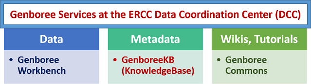
Genboree Account
If you are a new user, please follow the steps below to obtain a Genboree account and access to all associated services.
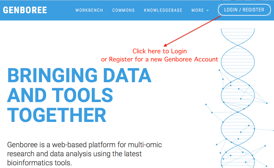
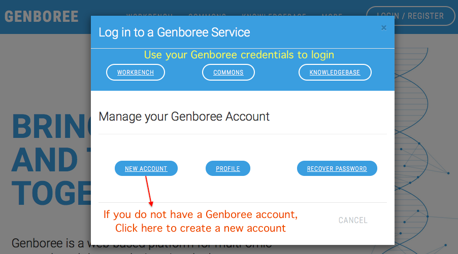
- Sign up for a Genboree Account: You can sign up for a new Genboree account at http://www.genboree.org/. Click the Login/Register button in the top right corner and then select New Account from the dialog. Fill out the registration form with your details and hit Submit. You'll get an email asking you to confirm (typical signup/verification process).
- Log into the Genboree Commons and GenboreeKB: Next, you will need to sign in once to the Genboree Commons (used for exRNA related communications) and GenboreeKB (used for navigating exRNA metadata). You should use the username and password obtained from Step 1. Signing in once allows our system to recognize you so we can add you to the appropriate projects/sub-projects. Sign into the Genboree Commons at http://genboree.org/theCommons/login and the GenboreeKB at http://genboree.org/genboreeKB/login.
- Email the BRL exRNA Team: Finally, you will need to email BRL to gain access to the appropriate projects/sub-projects on the Genboree Commons and GenboreeKB. We will also provide a dedicated, shared directory for your lab on our FTP server so that your lab can upload submissions for the DMRR data and metadata processing pipeline. Please include your Genboree username and PI when you email us.
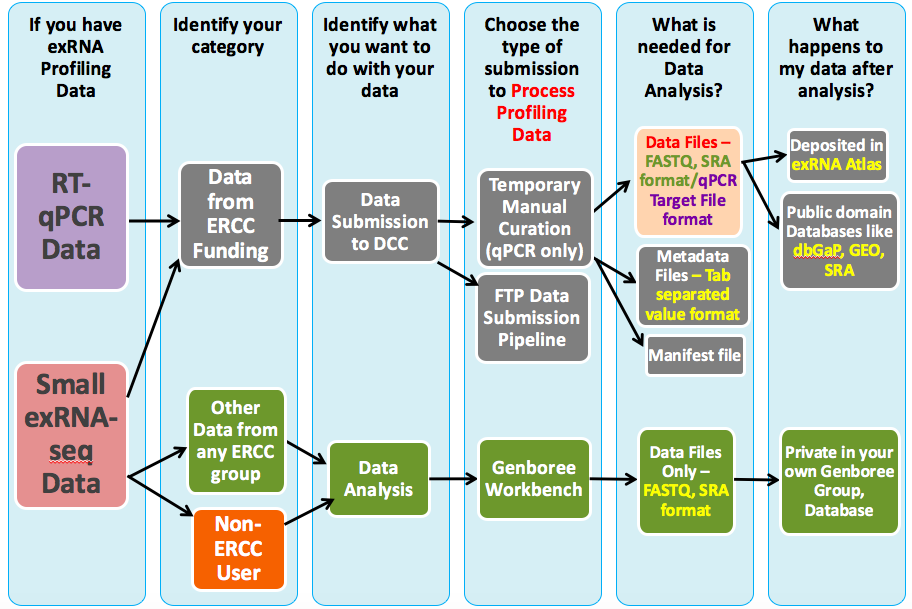
What Can I Do with exRNA Profiling Data?
The exRNA Atlas
The exRNA Atlas is the data repository of the ERCC. It includes exRNA profiles derived from various biofluids and conditions and currently stores data profiled from small RNA sequencing assays and RT-qPCR assays.
To learn more about the Atlas, you can read our tutorials:
Submitting Your Data to the Atlas
You can also learn more about submitting your own data to the Atlas via our Data Submission to DCC using FTP Wiki page.
All Atlas metadata is stored in the Genboree KnowledgeBase, a MongoDB-backed database curation service.
Our metadata models follow the exRNA Metadata Standards developed by the Metadata and Data Standards (MADS) Working Group of the ERCC.
Analyzing Your Own exRNA Data
If you'd like to analyze your own data using the tools developed by the ERCC, you can use the Genboree Workbench to do so.
The Genboree Workbench is a web-based platform for performing data analysis. You can upload your data and perform various analyses using a "drag and drop" user interface.
To get started using the Genboree Workbench, you can view our collection of introductory materials.
Once you understand the basics of using the Workbench, you can start using the different ERCC tools to analyze your exRNA data:
DMRR/DCC Demos at Meetings
- May 2014 - Demo of small and long RNA-Seq pipelines at the ERCC 2nd Investigators' Meeting, May 2014, at Bethesda, MD
- November 2014 - Demo of small RNA-seq pipeline and use cases presented at the ERCC 3rd Investigators' Meeting, November 2014, at Rockville, MD
- April 2015 - Demo of small RNA-seq pipeline and use cases presented at the ERCC 4th Investigators' Meeting and ISEV Annual Meeting, April 2015, at Bethesda, MD
- May 2015 - CIBR RNA-seq workshop - Demo of exceRpt small RNA processing pipeline, May 2015, at Baylor College of Medicine, Houston, TX
- November 2015 - Data Submission & Analysis Infrastructure at the DMRR - Talk at the ERCC 5th Investigators' Meeting, November 2015, at Rockville, MD
- April 2016 - DMRR Data Analysis and Bioinformatics Workshop - ERCC 6th Investigators' Meeting, April 2016, at Bethesda, MD
Prof. Aleksandar Milosavljevic - Principal Investigator
BRL Team - Point Person
Data Submission to dbGaP
The database of Genotypes and Phenotypes (dbGaP) was developed to archive and distribute the data and results from studies that have investigated the interaction of genotype and phenotype in Humans.
The ERCC Data Coordination Center developed this wiki to guide ERCC members on how to submit their data to dbGaP or GEO, after they have submitted their data to the exRNA Atlas.
To submit your data to dbGaP, follow these six steps:
1. Register the study
2. Fill out study config
3. Create phenotype data
4. Create sequence metadata file
5. Upload sequence file
6. Confirm and release the study
Please contact the ERCC DCC at brl-exrna@bcm.edu if any assistance is needed and we can help with steps 4-6.
We will need to be assigned as submitter for the study (the PI will have the option to do so after the study has been registered), and a completed submission to the exRNA Atlas.
Full Submission Guide From dbGaP
Full submission guide
Understanding the Process of Data Submission to dbGaP
Submission overview
Register Your Study
Finding the Genomic Program Administrator (GPA) and registering the study.
Fill Out the Study Config
What is the Study Config?
Here is a study config file with required areas highlighted in yellow.
Fill Out the Phenotype Data
Subject Consent Files
Sample Mapping Files
Pedigree Files
Subject Phenotypes Files
Sample Attributes Files
Molecular Data Submission
Molecular data should be submitted to the dbGaP Submission Portal under the section "Other files" with type "Molecular Data". It should be submitted along with the phenotype data.
For more information and other requirements, here is the FAQ from dbGaP
High Throughput Sequencing Submission
Once the previous files have been validated by dbGaP, the dbGap curator will reach out and provide the sequence metadata file to be filled and returned.
- Instructions are provided in the sequence metadata file.
Upload Sequence File
The sequence metadata file will have to be validated by dbGaP first and then the dbGaP curator will send the information on where to submit the sequence files.
Confirm and Release the Study
The dbGaP curator will provide preview of the study and make sure everything is correct prior to release it on dbGaP.
Overview of Data & Metadata Submission to the DCC (via FTP Pipeline)
This Wiki page includes instructions on how to submit your data (with accompanying metadata) to the Data Coordination Center (DCC)
using the Genboree FTP Data Submission Pipeline.
- If the dataset you are submitting is part of a new grant (ex. 4UH3TR000906-03) please email the grant number to DCC at brl-exrna@bcm.edu
If you're submitting small RNA-seq data, please follow the steps in the "Small RNA-seq Data Submission Pipeline" section.
If you're submitting long RNA-seq data, please follow the steps in the "Long RNA-seq Data Submission Pipeline" section.
If you're submitting qPCR data, please follow the steps in the "qPCR Data Submission" section.
Please contact us at brl-exrna@bcm.edu for guidance if you have a large data set (> 100GBs).
Prior to Your Submission
This tutorial will walk you through the entire process of creating an FTP account, formatting and submitting your data and metadata properly,
and then seeing your dataset on the Atlas.
Step 0: Create an FTP Account on the Genboree FTP Server
 Creating Your FTP Account
Small RNA-seq Data Submission Pipeline
All submitted samples will be processed through the exceRpt Small RNA-seq Pipeline for exRNA Profiling
and exceRpt Small RNA-seq Post-processing tools.
Files Needed for Data Submission
Your submission will consist of three different files:
- a data archive: The data archive will contain all of your different data files (FASTQ / SRA) as well as an optional spike-in file (FASTA) for those inputs.
- a metadata archive: The metadata archive will contain various metadata documents relating to your data submission.
- a manifest file: The manifest file will link together your data and metadata files, and it will also provide other valuable information for verifying that your submission is complete.
 IMPORTANT NOTE
All three files must have the same file name prefix ("samples" is the prefix in "samples_data"). Note that the data archive file name ends in _data, the metadata archive file name ends in _metadata, and the manifest file name ends in .manifest.json.
In this illustrative example, the submission files will be named like this:
- samples_data.zip
- samples_metadata.zip
- samples.manifest.json
In this example, "samples" was chosen as sample name. You should give a more descriptive name to your actual submission files ("gastricCancerOct2015_data.zip", for example).
Step 1: Preparing Your Data Archive
Prepare Your Data Archive
Prepare Your Metadata Archive
Step 3: Preparing Your Manifest File
Prepare Your Manifest File
Step 4: Uploading Your Submission to the FTP Server for Processing
Upload Submission to the DCC using FTP Server
Step 5: Processing Your Files
Processing Your Files
Long RNA-seq Data Submission Pipeline
Files Needed for longRNAseq Data Submission
Your submission will consist of three different files:
- a data archive: The data archive will contain all of your different paired-end reads FASTQ data files.
- a metadata archive: The metadata archive will contain various metadata documents relating to your data submission.
- a manifest file: The manifest file will link together your data and metadata files, and it will also provide other valuable information for verifying that your submission is complete.
IMPORTANT NOTE
All three files must have the same file name prefix ("samples" is the prefix in "samples_longRNAseqdata"), other than the data archive file name ending in _longRNAseq_data, the metadata archive file name ending in _longRNAseq_metadata, and the manifest file name ending in _longRNAseq.manifest.json.
In this illustrative example, the submission files will be named like this:
- samples_longRNAseq_data.zip
- samples_longRNAseq_metadata.zip
- samples_longRNAseq.manifest.json
In this example, "samples" was chosen as sample name. You should give a more descriptive name to your actual submission files ("gastricCancerOct2015_longRNAseq_data.zip", for example).
Step 1: Preparing Your longRNAseq Data Archive
Prepare Your longRNAseq Data Archive
Prepare Your longRNAseq Metadata Archive
Step 3: Preparing Your longRNAseq Manifest File
Prepare Your longRNAseq Manifest File
Step 4: Uploading longRNAseq Submission to the FTP Server for Processing
Upload longRNAseq Submission to the DCC using FTP Server
Step 5: Processing Your longRNAseq Files
Processing Your longRNAseq Files
qPCR Data Submission
Files Needed for qPCR Data Submission
Your submission will consist of two or three different files:
- a data archive: The data archive is OPTIONAL. It will contain all of your different data files (RDML format or any other custom format provided by the qPCR instrument).
- a metadata archive: The metadata archive will contain various metadata documents relating to your data submission.
- a manifest file: The manifest file will provide valuable information about your submission.
IMPORTANT NOTE
Both files must have the same file name prefix ("samples" is the prefix in "samples_data"), other than the data archive file name ending in _qPCR_data, the metadata archive file name ending in _qPCR_metadata, and the manifest file name ending in .manifest.json.
In this illustrative example, the submission files will be named like this:
- samples_qPCR_data.zip
- samples_qPCR_metadata.zip
- samples_qPCR.manifest.json
In this example, "samples" was chosen as sample name. You should give a more descriptive name to your actual submission files ("gastricCancerOct2015_qPCR_data.zip", for example).
Step 1: Preparing Your qPCR Data Archive
Prepare Your qPCR Data Archive
Prepare Your qPCR Metadata Archive
Step 3: Preparing Your qPCR Manifest File
Prepare Your qPCR Manifest File
Step 4: Uploading qPCR Submission to the FTP Server for Processing
Upload qPCR Submission to the DCC using FTP Server
Step 5: Processing qPCR Your Files
Processing Your qPCR Files
Submission to a Public Repository
Controlled-access data repository:
Data Submission to dbGaP
Public-access data repository:
Data Submission to GEO
Miscellaneous Tips and Tricks
Below, you'll find some useful tips and tricks for creating your submission for the FTP Pipeline.
Creating an Archive
Creating an Archive
Learning How to Use the Terminal
If you need help navigating the terminal (and want to learn some basic Linux/OSX commands), the following link will be useful:
Gene Expression Omnibus (GEO) is a public access data repository. It is a public functional genomics data repository supporting MIAME-compliant data submissions. Array- and sequence-based data are accepted.
The ERCC Data Coordination Center developed this wiki to guide ERCC members on how to submit their data to dbGaP or GEO, after they have submitted their data to the exRNA Atlas.
GEO submission requires filling out the metadata sheet for the submission.
Please follow the instructions from the full submission guide below for small/long RNAseq or qPCR.
The ERCC DCC can also facilitate the submission, please email us at brl-exrna@bcm.edu
We will require the following:
- GDS certificate from your institution,
- PI's GEO ID
- Release date for the dataset
- Completed submission to the exRNA Atlas.
Data Submission to GEO for Small/Long RNAseq
Full Submission Guide for Small/Long RNAseq From GEO
GEO Submission Guide for Small/Long RNA
Submission Requirements
Submit to GEO via FTP
- Sign in to GEO.
- Obtain the personalized space.
- Obtain the FTP server credentials (the password changes over time).
- Connect to the FTP host address via third-party software, FileZilla, etc.
- Navigate to the personalized space.
- Create a folder with a meaningful name in the personalized space.
- Upload the metadata sheet, processed data, and raw data files.
- Notify GEO.
- Select "Notify GEO about your FTP file transfer".
- Fill out the form after the files have been transferred.
Data Submission to GEO for qPCR
Full Submission Guide for qPCR From GEO
GEO Submission Guide for qPCR
Submission Requirements
- Filled out metadata sheet. qPCR metadata template
- Matrix non-normalized worksheet (second tab in the template).
- Matrix normalized worksheet (third tab in the template).
Make sure the amount of samples matches in the metadata sheet and the two matrices
- Sign in to GEO.
- Select "Transfer files to GEO with web form".
- Upload the metadata sheet and fill out the form.
Description of Domains
Within each template, the domain column gives you information about what kinds of values can be provided for each property.
Below, we describe what each of these domains mean.
autoID
The autoID domain indicates that our server can automatically generate a value for the associated property.
However, in our case, we'll go ahead and provide our own values instead of letting the server generate the values for us.
You can just follow the directions in the metadata submission guide to learn more.
bioportalTerm and bioportalTerms
The bioportalTerm and bioportalTerms domains indicate that your value will be validated against the the ontology (or ontologies) listed in the domain.
Generally, the value won't be validated against the entire ontology - it'll be validated against a subset (subtree) of the ontology.
The best way to validate your value is to use the GenboreeKB templates provided for each metadata type.
You will learn more about this process when creating your individual metadata files.
boolean
The boolean domain indicates that your value must either be true or false. Note that true and false are case-sensitive - you can't put TRUE, trUe, falSE, etc.
date
The date domain indicates that you must insert a date. This date should follow a particular format: YYYY/MM/DD. Example values include:
- 2017/04/13
- 2016/01/01
- 2016/03/12
enum
The enum domain indicates a group of possible values for that property. For example, the domain might look like:
- enum(Experimental, Control)
- enum(Dog, Cat, Human)
- enum(Add, Protect, Release)
The values inside the parentheses are the possible values for that property. If a property has enum(Experimental, Control) as its domain, for example,
then you must write Experimental or Control - any other value will be invalid. Note that the values ARE case-sensitive - you can't write experimental, conTrol, etc.
fileUrl
The fileUrl domain indicates that the provided value must be a URL directly pointing to a file of some kind. This URL must be complete. Example values include:
For any required properties, our metadata submission guide will give specific directions on how to fill out values for properties with this domain.
float
The float domain indicates that you must insert an float (integer / decimal) value for that property. Example values include:
floatRange
The floatRange domain specifics an (inclusive) float (decimal / integer) range under which your value must fall. For example, the domain might look like:
*floatRange(-5, 9)
*floatRange(-5.93,5.92)
*floatRange(0, 100.01)
So, if my domain is floatRange(-5,9), I can put any value between -5 and 9 (inclusive). This could be -5, -1.2, 0, 8.59, 9, or many other values.
gbAccount
The gbAccount domain indicates that the provided value should be a Genboree account name.
We will then automatically use that account name to fill in associated information.
int
The int domain indicates that you must insert an integer value for that property. Example values include:
intRange
The intRange domain specifics an (inclusive) integer range under which your value must fall. For example, the domain might look like:
*intRange(5, 9)
*intRange(-5,5)
*intRange(0, 100)
So, if my domain is intRange(5,9), that means my value must be 5, 6, 7, 8, or 9.
labelUrl
The labelUrl domain specifies a label and then a URL associated with that label. The formatting looks like: label|URL. Your URL can be relative or complete. Some example values include:
This domain can be useful because it supplies information to us about how a given website should be labeled.
measurement
The measurement domain indicates that you must insert a number followed by a valid measurement unit. For example, the domain might look like:
- measurement(years)
- measurement(nm)
- measurement(days)
For a given measurement, we accept the listed unit (years) as well as any comparable (inter-convertible) units, like days, months, hours, etc.
Thus, if a property has measurement(years) as its domain, then you could write 10 years, 5 days, 3 months, 2 hours, etc. It should be a specific number and not a range.
numItems
The numItems domain indicates that the associated property is an item list. The value for the property will be the number of items in the item list.
For example, imagine I have a property, * Authors, which is an item list, and it has 5 items (*- Author Name). This means the value for the * Authors property will be 5.
We actually automatically update the value for any property with the numItems domain, so you can leave the value blank if you want.
negFloat
The negFloat domain indicates that you must insert a negative float (integer / decimal) value for that property. You can also put 0. Example values include:
negInt
The negInt domain indicates that you must insert a negative integer value (or 0) for that property. Example values include:
omim
The omim domain indicates that the value must be an ID from the OMIM database at http://omim.org/.
We will then automatically use that ID to fill in associated information for that reference.
pmid
The pmid domain indicates that the value must be an ID from the PubMed database at http://www.ncbi.nlm.nih.gov/pubmed.
We will then automatically use that ID to fill in associated information for that publication.
posFloat
The posFloat domain indicates that you must insert a positive float (integer / decimal) value for that property. You can also put 0. Example values include:
posInt
The posInt domain indicates that you must insert a positive integer value (or 0) for that property. Example values include:
regexp
The regexp domain indicates that any value for the domain must meet the specified regular expression. Example domains include:
- regexp(EXR-[A-Z0-9]{6}-SUB)
- regexp(EXR-[A-Z0-9]{6}-PI)
- regexp(EXR-[a-zA-Z0-9]{6,}-ST)
These domains might look complicated, but our metadata submission guide will give specific directions on how to fill out values for required properties with this domain.
string
The string domain indicates that any text is acceptable (letters, numbers, etc.). Example values include:
- William Thistlethwaite
- 783123421
- Biomarker GD9103XZ*_*593
As you can see, you can pretty much put anything!
timestamp
The timestamp domain indicates that you must insert a timestamp. This timestamp should follow a particular format: YYYY/MM/DD XX:XX AM/PM. Example values include:
- 2017/04/13 09:30 AM
- 2016/01/01 12:12 PM
- 2016/03/12 12:15 AM
url
The url domain indicates that some kind of URL must be provided as a value. This URL can either be complete or relative. Example values include:
The first example above is a relative URL, while the second example is a complete URL.
For any required properties, our metadata submission guide will give specific directions on how to fill out values for properties with this domain.
[valueless]
The [valueless] domain indicates that you cannot insert a value for that property (it must remain blank).
These kinds of properties are used as section headers, for the most part.
The property name describes the content of the subproperties nested below - thus, it's not necessary to provide a value for the property.
Downloading Datasets from the exRNA Atlas
There are several different options for downloading datasets from the exRNA Atlas.
You can either download the datasets individually (on a per-sample basis), or you can download the datasets in bulk.
Downloading Individual Core Result Archives
Take a look at the following faceted search grid (certain metadata columns are hidden for this example):
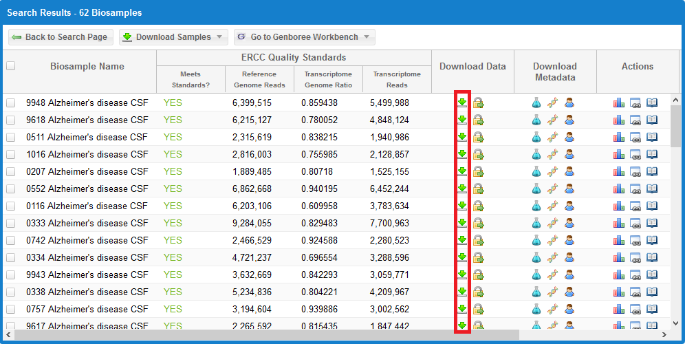
You can click the  icon for any given sample to download its core results archive.
This core results archive contains all of the most important files generated by the exceRpt pipeline, including all of the read mapping documents to various libraries.
Downloading Individual Raw FASTQ Data Files
Alternatively, if you want to download the raw FASTQ data file associated with a given sample, take a look at the following faceted search grid:
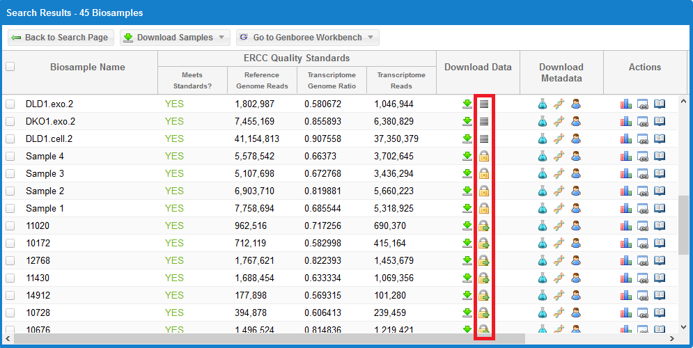
You can see three different icons in the highlighted column:
- The
 icon indicates that the raw FASTQ file is openly available for download.
This icon will only be present if the dataset is already available in a public domain archive like SRA or GEO.
Simply click the icon to download the raw FASTQ file.
- The
 icon means that the data is restricted access and is currently under the protected period (embargo).
The embargo on this dataset will end 12 months after the time the data was submitted to the DCC. View the ERC Consortium Data Access Policy for more details.
- The
 icon means that the data is deposited in the controlled access dbGaP archive.
You can click the  icon under the Actions column to view the dbGaP Study Id. You can then contact the PI through dbGaP to get access to the raw FASTQ data files.
Downloading Datasets in Bulk
If you want to download result files in bulk for a given search, you can click the Download Samples button at the top of the grid, as seen below:
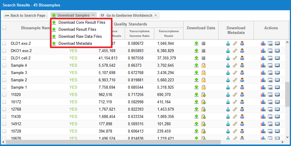
You can then choose between four different options.
The Download All Core Result Files link will download a tab-delimited file that contains information on how to download the processed core results archives for each sample.
The Download All Result Files link will download a tab-delimited file that contains information on how to download the full results archives for each sample.
These archives can be very large (gigabytes), so we recommend that you start by downloading the core results archives (which are usually around 3-5 MB).
The Download All Raw Data Files link will download a tab-delimited file that contains information on how to download all available raw sequencing data files in FASTQ format.
These FASTQ files are only available for samples that are open access.
You can tell which samples have available FASTQ files by looking for the icon in the Download Data column.
These tab-delimited files will contain two separate columns:
- The first column contains the names of the different samples.
- The second column contains the URLs to actually download the files.
There are several ways of downloading the files in your tab delimited list:
- You can copy and paste each URL in your browser and hit Enter to download each file in this list.
- For more advanced users, you can use a command line program like wget to download these files.
- wget -O {FILE NAME in Column 1} {URL in Column 2}, or
- curl --output {FILE NAME in Column 1} {URL in Column 2}
- Replace {FILE NAME in Column 1} with the actual file name in Column 1, and replace {URL in Column 2} with the actual URL in column 2.
In order to download one of these tab-delimited files, you must agree to the ERC Consortium Data Access Policy, which pops up in a new window.
This same policy can also be found at the top of each tab-delimited file.
The Download Metadata link in the Download Samples menu will download the biosample, donor, and experiment metadata documents associated with a single sample.
All metadata documents will be placed in a single text file.
Before downloading your metadata, you must select a single sample by using the checkboxes to the left of each sample in the grid.
Multiple sample selection is currently not allowed.
There are several different options for downloading data from the exRNA Atlas.
You can either download data on an individual, sample-by-sample basis, or you can download data in bulk.
Downloading Individual Core Result Archives
Take a look at the following faceted search grid (certain metadata columns are hidden for this example):
You can click the icon for any given sample to download its core results archive.
This core results archive contains all of the most important files generated by the exceRpt pipeline, including all of the read mapping documents to various libraries.
Downloading Individual Raw FASTQ Data Files
Alternatively, if you want to download the raw FASTQ data file associated with a given sample, take a look at the following faceted search grid:
You can see three different icons in the highlighted column:
- The icon indicates that the raw FASTQ file is openly available for download.
This icon will only be present if the dataset is already available in a public domain archive like SRA or GEO.
Simply click the icon to download the raw FASTQ file.
- The icon means that the data is restricted access and is currently under the protected period (embargo).
The embargo on this dataset will end 12 months after the time the data was submitted to the DCC. View the ERC Consortium Data Access Policy for more details.
- The icon means that the data is deposited in the controlled access dbGaP archive.
You can click the icon under the Actions column to view the dbGaP Study Id. You can then contact the PI through dbGaP to get access to the raw FASTQ data files.
Downloading Datasets in Bulk
If you want to download result files in bulk for a given search, you can click the Download Samples button at the top of the grid, as seen below:
You can then choose between four different options.
The Download All Core Result Files link will download a tab-delimited file that contains information on how to download the processed core results archives for each sample.
The Download All Result Files link will download a tab-delimited file that contains information on how to download the full results archives for each sample.
These archives can be very large (gigabytes), so we recommend that you start by downloading the core results archives (which are usually around 3-5 MB).
The Download All Raw Data Files link will download a tab-delimited file that contains information on how to download all available raw sequencing data files in FASTQ format.
These FASTQ files are only available for samples that are open access.
You can tell which samples have available FASTQ files by looking for the icon in the Download Data column.
These tab-delimited files will contain two separate columns:
- The first column contains the names of the different samples.
- The second column contains the URLs to actually download the files.
There are several ways of downloading the files in your tab delimited list:
- You can copy and paste each URL in your browser and hit Enter to download each file in this list.
- For more advanced users, you can use a command line program like wget to download these files.
- wget -O {FILE NAME in Column 1} {URL in Column 2}, or
- curl --output {FILE NAME in Column 1} {URL in Column 2}
- Replace {FILE NAME in Column 1} with the actual file name in Column 1, and replace {URL in Column 2} with the actual URL in column 2.
In order to download one of these tab-delimited files, you must agree to the ERC Consortium Data Access Policy, which pops up in a new window.
This same policy can also be found at the top of each tab-delimited file.
The Download Metadata link in the Download Samples menu will download the biosample, donor, and experiment metadata documents associated with a single sample.
All metadata documents will be placed in a single text file.
Before downloading your metadata, you must select a single sample by using the checkboxes to the left of each sample in the grid.
Multiple sample selection is currently not allowed.
Downloading Data from the exRNA Atlas
There are several different options for downloading data from the exRNA Atlas.
You can either download data on an individual, sample-by-sample basis, or you can download data in bulk.
Downloading Individual Core Result Archives
Take a look at the following faceted search grid (certain metadata columns are hidden for this example):
You can click the icon for any given sample to download its core results archive.
This core results archive contains all of the most important files generated by the exceRpt pipeline, including all of the read mapping documents to various libraries.
Downloading Individual Raw FASTQ Data Files
Alternatively, if you want to download the raw FASTQ data file associated with a given sample, take a look at the following faceted search grid:
You can see three different icons in the highlighted column:
- The icon indicates that the raw FASTQ file is openly available for download.
This icon will only be present if the dataset is already available in a public domain archive like SRA or GEO.
Simply click the icon to download the raw FASTQ file.
- The icon means that the data is restricted access and is currently under the protected period (embargo).
The embargo on this dataset will end 12 months after the time the data was submitted to the DCC. View the ERC Consortium Data Access Policy for more details.
- The icon means that the data is deposited in the controlled access dbGaP archive.
You can click the icon under the Actions column to view the dbGaP Study Id. You can then contact the PI through dbGaP to get access to the raw FASTQ data files.
Downloading Datasets in Bulk
If you want to download result files in bulk for a given search, you can click the Download Samples button at the top of the grid, as seen below:
You can then choose between four different options.
The Download All Core Result Files link will download a tab-delimited file that contains information on how to download the processed core results archives for each sample.
The Download All Result Files link will download a tab-delimited file that contains information on how to download the full results archives for each sample.
These archives can be very large (gigabytes), so we recommend that you start by downloading the core results archives (which are usually around 3-5 MB).
The Download All Raw Data Files link will download a tab-delimited file that contains information on how to download all available raw sequencing data files in FASTQ format.
These FASTQ files are only available for samples that are open access.
You can tell which samples have available FASTQ files by looking for the icon in the Download Data column.
These tab-delimited files will contain two separate columns:
- The first column contains the names of the different samples.
- The second column contains the URLs to actually download the files.
There are several ways of downloading the files in your tab delimited list:
- You can copy and paste each URL in your browser and hit Enter to download each file in this list.
- For more advanced users, you can use a command line program like wget to download these files.
- wget -O {FILE NAME in Column 1} {URL in Column 2}, or
- curl --output {FILE NAME in Column 1} {URL in Column 2}
- Replace {FILE NAME in Column 1} with the actual file name in Column 1, and replace {URL in Column 2} with the actual URL in column 2.
In order to download one of these tab-delimited files, you must agree to the ERC Consortium Data Access Policy, which pops up in a new window.
This same policy can also be found at the top of each tab-delimited file.
The Download Metadata link in the Download Samples menu will download the biosample, donor, and experiment metadata documents associated with a single sample.
All metadata documents will be placed in a single text file.
Before downloading your metadata, you must select a single sample by using the checkboxes to the left of each sample in the grid.
Multiple sample selection is currently not allowed.
Overview
Introduction to the exRNA Atlas
The exRNA Atlas is the data repository of the Extracellular RNA Communication Consortium (ERCC), which includes small RNA sequencing and qPCR-derived exRNA profiles from human and mouse biofluids.
All RNA-seq datasets are processed using version 4 of the exceRpt small RNA-seq pipeline and ERCC-developed quality metrics are uniformly applied to these datasets.
There are two different versions of the exRNA Atlas:
- a public version (accessible by everyone) and
- a private version (accessible only by ERC Consortium members).
- The private version of the Atlas stores additional exRNA profiles that are not yet available to the public.
- You must log into your Genboree account in order to access the private version of the Atlas.
- If you are a member of the ERC Consortium and are unable to log in to the private atlas, please contact the Data Coordination Center (brl-exrna@bcm.edu) for assistance.
If you are interested in submitting data to the Atlas, visit the Data & Metadata Processing Guide page to learn more about the submission process.
Selecting Profiles
ncRNA Search Bar
Using the ncRNA Search Bar
Faceted Charts
Viewing Selected Biosamples in Grid via Faceted Charts
Biosample Partition Grids
Viewing Biosamples in Biosample Partition Grid
Drill-down Sub-setting of Biosamples via Linear Tree
Viewing Selected Biosamples in Grid via Linear Tree
Downloading Data and Metadata from the exRNA Atlas
Viewing exRNA Profiling Datasets
Viewing exRNA Profiling Datasets
Viewing Atlas Statistics
Viewing Atlas Statistics
Running Analyses and Viewing Analysis Results Using the exRNA Atlas
Running Analyses and Viewing Analysis Results Using the exRNA Atlas
BedGraphs
BedGraphs are publicly accessible, base pair level coverage maps of the genome and are present for every sample in the exRNA atlas. You can find them inside the CORE_RESULTS archives for any sample within a study (studies are defined by an accession such as EXR-TEST1-AN) . There will be 3 bedGraph files you can use
- endogenousAlignments_genome_Aligned.bedgraph.xz - Shows where reads that aligned to the host genome fell
- endogenousAlignments_genomeUnmapped_transcriptome_Aligned.bedgraph.xz - Has reads that did not align to the host genome
- endogenousAlignments_genomeMapped_transcriptome_Aligned.bedgraph.xz - Shows where reads that aligned to the host genome fell in the transcriptome
Data Slicing
You can select regions of interest across the genome and samples of interest across any study present in the atlas and perform "data slicing" and retrieve a matrix with the coverage of your regions (rows) per sample (columns) by using the downloadable exRNA Data Slicer tool found here.
Genome browser
You can view which regions are detected in the atlas using the UCSC genome browser. These coverage files have been split by biofluid and library preparation kit i.e. you can see regions of the genome where at least one plasma samples processed by the TruSeq library preparation kit has reads. We provide two coverage cut offs: 1 read and 5 reads. Files can also be downloaded here.
RNA binding proteins (RBPs)
- For the publicly available 150 RBPs where ENCODE/ENCORE have performed eCLIP (a method to determine where a protein binds across the genome), we have intersected regions bound by the RBPs with exRNA reads. Two versions of files where the RBP binding regions are present are available. All of these files are present inside each study (an accession EXR-TEST1-AN). Please note though there are 150 RBPs, there will be 296 files. This occurs because ENCODE/ENCORE profiled the RBPs in one OR two different cell lines. For RBPs profiled in 1 cell line there is only one file. For those profiled in two cell lines there are 3 files = one for HepG2, one of K562, and one for a merged file where we have merged regions found in both cell lines.
1) For each study, you can view reads that fall into a give RBP's binding sites across samples. You can find these in the postProcessedResults files. Through the atlas datasets page, you can download All Summary Files using the download icon in the bottom right of each dataset card or you can access them through the FTP. There is a folder name _intersect_individual_RBP.combined_samples.tgz which houses the RBP coverage files for that study.
2) For each sample, you can look at coverage of reads that fall into all 150 RBPs. On the atlas, you can select samples in the sample viewer and download the Core Results Archives - inside the fastq folder there will be a endogenousAlignments_genome_Aligned_intersect_individual_RBP.tgz folder which houses the 96 files for each sample. These regions have been intersected so if RBP A binds to chromosome 1, 1:10 and RBP B binds to chromosome 1, 5:15 then three regions will be created 1:5, 5:10, and 10:15. In these files, the rows are the overlapping regions and the columns are for each RBP.
exRBPs
- For the publicly available 150 RBPs where ENCODE/ENCORE have performed eCLIP (a method to determine where a protein binds across the genome), we have intersected regions bound by the RBPs with exRNA reads. Two versions of files where the RBP binding regions are present are available. Please note though there are 150 RBPs, there will be 296 files. This occurs because ENCODE/ENCORE profiled the RBPs in one OR two different cell lines. For RBPs profiled in 1 cell line there is only one file. For those profiled in two cell lines there are 3 files = one for HepG2, one of K562, and one for a merged file where we have merged regions found in both cell lines.
1) For each study, you can view reads that fall into a give RBP's binding sites across samples. You can find these in the postProcessedResults files. Through the atlas datasets page, you can download All Summary Files using the download icon in the bottom right of each dataset card or you can access them through the FTP. There is a folder name _intersect_individual_RBP.combined_samples.tgz which houses the RBP coverage files for that study.
2) For each sample, you can look at coverage of reads that fall into all 150 RBPs. On the atlas, you can select samples in the sample viewer and download the Core Results Archives - inside the fastq folder there will be a endogenousAlignments_genome_Aligned_intersect_individual_RBP.tgz folder which houses the 96 files for each sample. These regions have been intersected so if RBP A binds to chromosome 1, 1:10 and RBP B binds to chromosome 1, 5:15 then three regions will be created 1:5, 5:10, and 10:15. In these files, the rows are the overlapping regions and the columns are for each RBP.
The exRNA Atlas Explorer tool allows you to visualize the RBPs across any dataset or sets of datasets in the atlas. The tool is available here
Learn More About the exceRpt small RNA-seq Data Analysis Pipeline
exceRpt Homepage
Genboree Tutorial for Using exceRpt
Understanding Your exceRpt Results
exceRpt Version Updates
exRNA Atlas v3
Using ~6500 exRNA profiles from human serum, plasma, cerebrospinal fluid, urine and saliva across 60 datasets, this study identifies >30 million unique extracellular Genomic Loci (exGLs) covering >18% of the human genome expressing exRNA.
extracellular Genomic Loci (exGLs) and associated annotations
Overview
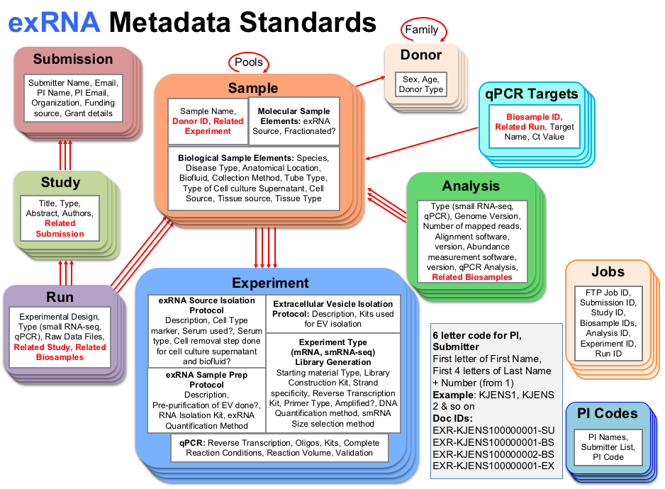
The infographic below will give you a better sense of how the different documents in the exRNA GenboreeKB relate to one another.
As an example, we see that any document in the "Study" collection will have a connection to a Submission document in its "Related Submissions" item list.
In other words, if you have a "Study" document, you must have a related "Submission" that the "Study" document falls under. Connections between collections
are made apparent through the use of red arrows and the red text within each collection's attributes ("Related Submission" for the "Study" collection, for example).
Note that the attribute list given in the infographic is merely a summary - you can look at the respective schema / templates for each collection below
to get a full list of the different properties that a given document within that collection will contain.
Finally, the box in the lower right corner of the infographic gives some information about how each document is named.
More details about how individual documents are named can be found in the exRNA Metadata Documents Accession section below.
Refer to the Prepare your Metadata Archive Wiki for more details.
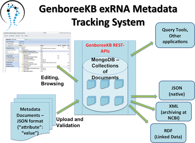
If you want to learn more about how the exRNA GenboreeKB works, you should check out the introductory materials here.
Below, you'll see some key features of our exRNA GenboreeKB Metadata Tracking System:
- Front end User Interface - Redmine (Ruby-on-rails) application plug-in
- Back end Database - MongoDB
GenboreeKB = Multiple Collections of Documents
- Each metadata collection has its own document data model
- Singly-Rooted Nested Collection of Properties
- Data model - Defines “properties” and “property definitions”
- Property Definitions - Fields describing each property like “domain”, “required”, “identifier”, “category”, “description”, etc
- Key Features -
- Browse, Manage documents
- Browse, Manage data models
- Queries
- Views
- Bulk upload of documents in JSON/Tabbed formats
- Bulk download of documents in JSON/Tabbed formats
- Dynamic retrieval and validation of ontology terms from Bioportal
Extracellular Genomic Loci (exGLs) and associated annotations
Previous versions of the exRNA Atlas focused on distinct aspects of exRNA biology. The first version mapped exRNA to its vesicular (exosomes and other extracellular vesicles) and non-vesicular (lipoproteins, RNPs, and other specific classes particles) carriers in human biofluids, and the second version further deepened our understanding of exRNA carriers by identifying extracellular RNA-binding proteins (exRBPs) that associate with exRNA fragments in the extracellular space. One key limitation of those early maps was that the exRNA expression was quantitatively ascertained using GENCODE and ENCODE/ENCORE genome annotations. While being useful as initial stepping stones toward understanding exRNA biology, these annotations heavily constrained the insights that could be gained about the role of exRNA in human biology.
The most glaring gap in exRNA biology was the lack of information about the loci that are transcribed into exRNA. With the completion of the Extracellular RNA Communication Consoritum and aggregation of the uniformly processed exRNA profiles in the Atlas, we here addressed this question for the first time. We provide the first map of extracellular Genomic Loci (exGLs) transcribed and exported as extracellular RNA into human plasma, serum, urine, cerebrospinal fluid (CSF), and saliva. These five biofluids were selected because they represent the largest number of samples in the exRNA Atlas, comprising 6,532 smRNA-seq profiles from 60 datasets. For those biofluids, we identify biofluid-specific exGLs de novo, independent of previous genome annotations. This study identifies >30 million unique extracellular RNA genomic loci (exGLs) covering >18% of the human genome expressing exRNA.
All exGLs are viewable via UCSC Genome Browser track hub
ExRNA Atlas datasets used to generate exGLs are available here
To support standardized referencing of these exGLs, we developed the exGL identification service, which assigns unique identifiers (exGLids) to each exGL. exGLids and associated annotations—such as expression depth, gene or regulatory element overlap, and biofluid distribution—can be accessed via User Interface or programmatically via APIs or as TSVs
Overview
To learn the basics of GenboreeKB, view the documentation found here.
In brief, we use GenboreeKB to store the metadata documents associated with samples present in the exRNA Atlas.
The GenboreeKB UI allows you to view those documents. It also allows you to edit documents, find ontology terms for properties, and
experiment with different documents while assembling your metadata submission for the FTP submission pipeline.
Each GenboreeKB is associated with a different group of metadata documents.
There are three different relevant KBs:
- Public Atlas KB
- Private Atlas KB
- "Testing Ground" Scratch KB
- Members of the public will only be able to access the public Atlas KB.
- Public users cannot write to the public Atlas KB.
- This means that they cannot upload new documents, edit existing documents, etc.
- All they can do is browse (the public Atlas).
- ERCC members can access all three KBs.
- They can write to the private Atlas KB and the "Testing Ground" KB, but they cannot write to the public Atlas KB.
- Only ERCC administrators can write to the public Atlas KB.
- ERCC members should use the "Testing Ground" KB for all scratch work when preparing their metadata documents for submission to the FTP Pipeline.
- This includes searching for ontology terms, checking the validity of a given document, and anything else that comes to mind.
- ERCC members should not use the private Atlas KB for scratch work.
- The only reason to edit documents in the private Atlas is to fix errors and provide updates (users should not upload new documents).
- If a user updates a document in the private Atlas and wants that document uploaded to the public Atlas, he/she should let the DCC admins (Emily) know.
Step-by-step Instructions to Navigate to the Relevant GenboreeKB
In order to better understand the collections you will be browsing, refer to the Wiki page exRNA Metadata Standards.
1. Login
- Log in to GenboreeKB using your Genboree user name and password.
- If you are a member of the ERCC, you will be able to access both the public Atlas and private, ERCC-only Atlas.
- In order to get access to the private Atlas KB, you will need to contact Emily after you login for the first time.
- One of us will grant you permission to see the private Atlas KB in your Projects page.
- Non-ERCC members can only access the public Atlas.
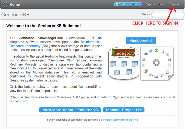
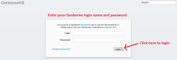
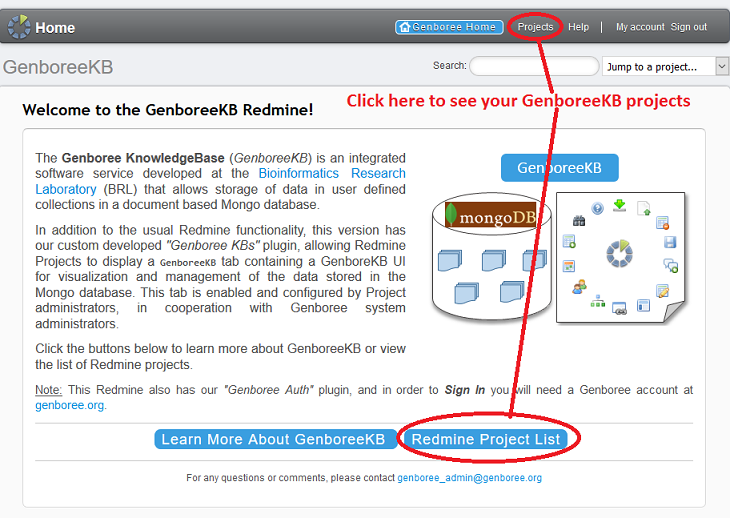
2. Navigate to the Relevant KB
Each Atlas (public and private) has its own GenboreeKB Project.
In order to navigate to the public Atlas, click the 'Extracellular RNA Atlas' project.

In order to navigate to the private Atlas (if you're an ERCC member), expand the 'exRNA Metadata Standards' project
and select the 'Extracellular RNA Atlas - Consortium' subproject. You can also select the "Testing Ground" Scratch KB
by selecting the 'exRNA Metadata - Templates' subproject.

Regardless of which KB you choose, click the 'GenboreeKB' button at the top of the page to navigate to the GenboreeKB UI.
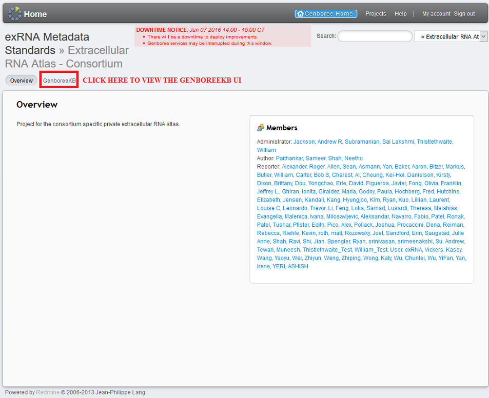
3. View General Stats About the Current KB
When you enter a given KB, you will see a summary page consisting of several charts and graphs.
These diagrams will contain general statistics about that KB, such as number of docs per collection,
total number of docs over time, and number of doc edits over time.

At the top of the KB UI, there will be a Collection menu that will allow you to choose between the different collections for that KB.
Each collection has its own unique document model and set of documents.
We can see an example of the available collections for the private Atlas (as of 6/16/16) in the picture below:
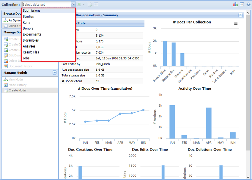
For example, all biosample documents can be found in the Biosamples collection.
After we select a collection (Biosamples, for example), we'll be given statistics on that collection, as seen below:

After you have selected your collection of interest, your next action will depend on what you want to accomplish.
Do you want to browse the existing documents, or edit an existing document, or add a new document?
We will explain how to complete these tasks below.
Once you've selected your metadata collection, you might want to create a new document.
You should only create a new metadata document using the Testing Ground Scratch KB.
You should not create any new metadata documents in the private Atlas or public Atlas.
Each document you create will have its own, unique document identifier (doc ID).
You can either create your own doc ID, following a collection-specific format described below,
or you can allow the GenboreeKB UI to automatically generate your doc ID for you.
If you want to create your own doc ID, follow the directions in the Creating a Valid Document Identifier section.
Please note that if the KB UI automatically generates your doc ID, that ID will not contain your PI ID (a necessary part of any doc ID that goes into the Atlas).
However, the FTP Pipeline will automatically insert this PI ID for you when processing your documents, so the final version that ends up in the private or public Atlas
will contain the PI ID. In other words, don't worry about the fact that your auto-generated doc ID doesn't include your PI ID!
Creating a Valid Document Identifier
If you would prefer to have the GenboreeKB UI automatically generate your doc ID, you can ignore this section.
All identifiers must begin with EXR-, regardless of collection.
Then, you should provide your PI ID followed by 6 alphanumeric characters (numbers and capital/lowercase letters).
Your PI ID can be found in a couple of different ways:
- Look at the name of your lab's FTP directory. The last part of the name will be a lowercase version of your PI ID.
- Example: If my FTP directory is "exrna-amilo1", then my PI ID is AMILO1.
- Download the collection of docs found here and find your PI in the list.
- We recommend searching for your PI's last name. It will be associated with the "- PI Last Name" subproperty of a document.
Look at the value of the "ERCC PI Code" root property right above the "- PI Last Name" subproperty.
The middle part of this identifier will be your PI ID.
- Example: If my PI's last name is Milosavljevic, I would search for that name. The associated document identifier is EXR-AMILO1-PI,
so my PI ID is AMILO1.
- If your PI is missing from the list, please let "Emily know so we can add him/her.
Finally, you will need to write another dash (-) followed by the collection suffix associated with your collection.
A table containing collection types, suffixes, and example identifiers can be found below:
Examples
| Type |
Suffix |
Example Accession |
| Biosample |
BS |
EXR-KJENS12P3L78-BS |
| Donor |
DO |
EXR-KJENS12P3L78-DO |
| Experiment |
EX |
EXR-KJENS12P3L78-EX |
| Analysis |
AN |
EXR-KJENS12P3L78-AN |
| Submission |
SU |
EXR-KJENS12P3W78-SU |
| Run |
RU |
EXR-KJENS12P3W78-RU |
| Study |
ST |
EXR-KJENS12P3L78-ST |
| File |
FL |
EXR-KJENS12P3L78-FL |
Your identifier must also be unique - no other document in that collection can have the same identifier.
Creating a New Document Through the UI
There are three different options for creating a new document through the UI. They can be seen below:
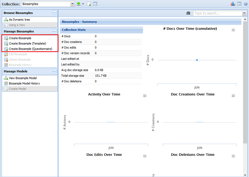
The most basic option is to create your metadata document without a template or questionnaire.
When you select this option, you will be prompted to provide a doc ID.
You can either provide your own doc ID (explained above) or leave the entry box blank and click OK.
If you leave the entry box blank, the doc ID will be automatically generated for you once you save the document.
When you create a document using the most basic option, only required properties will be present in the document initially.
You can always add other, optional properties though!
You can also use a template to create your document (if the collection has templates available).
Select the second option highlighted in the red box above and then choose the template you want to follow.
The template will contain all required properties as well as any recommended optional properties.
Finally, you can use a questionnaire to create your document (if the collection has questionnaires available).
Select the third option highlighted in the red box above and then choose the questionnaire you want to use.
By answering the series of questions presented, you will fill out the required fields in your document.
You will then only have to fill out any optional fields you want to include.
You don't need to use the UI to create a new metadata document - you can also upload a new, previously-made document.
Click the "Upload Documents" button near the top of the GenboreeKB panel.
You will then find the document you want to upload by clicking "Select File...".
If you are using the templates and other materials provided on this Wiki for creating documents, you should choose
the "TABBED - Compact Property Names" format.
Click "Upload" and then wait until you receive an email informing you that your document was successfully uploaded.
If the document fails validation, you will receive information in your email telling you how to fix your document.
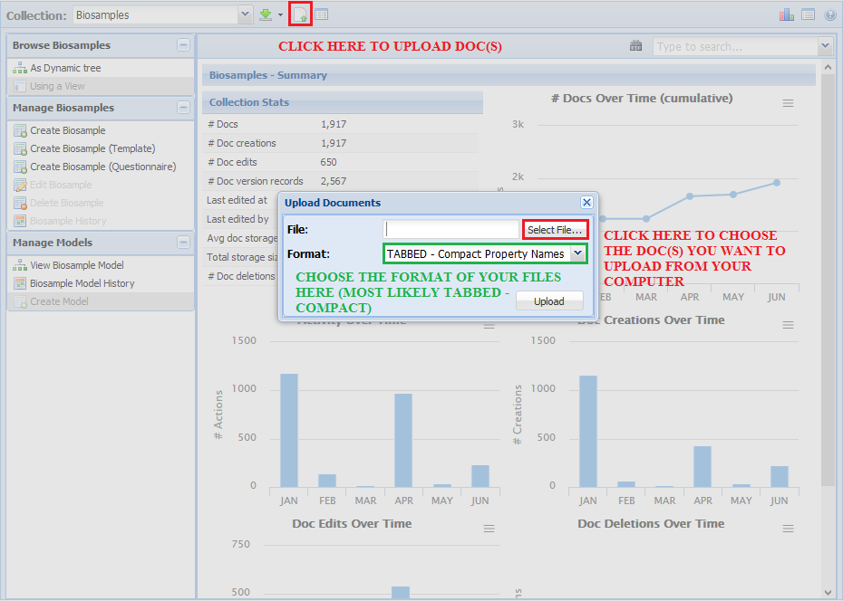
If you want to find an existing metadata document (instead of creating a new one),
you can either use the search toolbar in the top right corner of the UI window, or you can
query the collection.
The most straight-forward way of finding a document is to use the search toolbar.

If you know the doc ID of the document you're looking for, you can simply type it into
the search bar. You can also type part of the ID, and all matching results will show up.
For example, if I was interested in documents from the PI ID AMILO1, I could type
AMILO1 into the search bar and see a list of documents from AMILO1 in that collection.
Clicking the downward arrow to the right of the search bar will bring up your list of results
in case you search a given term and then click elsewhere, thus minimizing the list.
If the search bar is blank and you click this arrow, a list of random documents will be
displayed. This is useful if you don't know what you want to search for or don't understand
the doc ID format for a particular collection.
Please note that if there are many documents that match your search term, not all will be
listed. Thus, you'll need to use a different search feature (like the query described below)
in order to view a list of all matching documents.
Querying the Collection
Another way of finding a document of interest is using the query functionality found here:
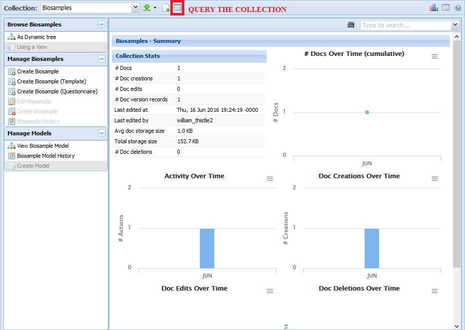
There will be a number of different options in the dialog window:
For the Query option, you can choose between Document ID and Indexed Properties.
- Document ID will search for a given term against the doc IDs present in the collection.
- Example: If I wanted to search for AMILO1 in the collection's doc IDs, I would pick this option.
- Indexed Properties will search for a given term in the indexed properties in the collection.
- You can find out which properties are indexed by going to the collection's model and looking at the 'index' column.
- Example: If I wanted to search for "Urine" for the "--- Biofluid Name" property in the Biosamples collection, I would
pick this option. Note that the "--- Biofluid Name" property is indexed.
For the Mode option, you can choose between Exact, Full, Keyword, and Prefix.
- Exact means that your search term has to exactly match the value of the property (case sensitive).
- Example: My search term "Urine" would match a property value of "Urine" but not "urine" or "urine and csf".
- Full means that your search term has to fully match the value of the property (case insensitive).
- Example: My search term "Urine" would match a property value of "Urine" and "urine" but not "urine and csf".
- Keyword means that your search term can be anywhere in the value of the property (case insensitive).
- Example: My search term "Urine" would match "Urine", "urine", and "urine and csf".
- Prefix means that your search term will match any property value that begins with your search term (case insensitive).
- Example: My search term "Urine" would match "Urine", "urine", and "urine and csf", but would not match "csf and urine".
For the View option, you can choose between different views that have been created by the DCC administrators for that collection.
- The different views will allow you to view different information in your search results.
- Example: One view might just show me the doc IDs of the docs that contain my search term, while another view
might additionally include biofluid name, disease type, and/or anatomical location.
For the Term option, you should write your search term.
When you click Submit, you can choose to see your search results in the current tab or in a new tab.
Once you've selected a metadata document, you'll be able to see its contents in the GenboreeKB UI window.
In particular, each document starts off "minimized", with only the root property and its immediate sub-properties displayed.
In order to see all of the sub-properties in a given document, right click on the root property ("Biosample" in the example below)
and click "Fully Expand". You can also right click a sub-property and click "Fully Expand" if you only want to expand that sub-property.
You can also click "Fully Collapse" if you want to minimize a given sub-property (or the doc as a whole).
Here, we see a document that has not been fully expanded:
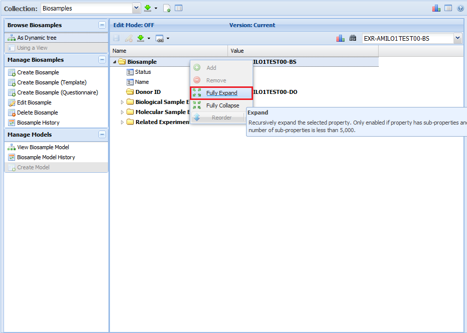
Now, the document has been fully expanded:
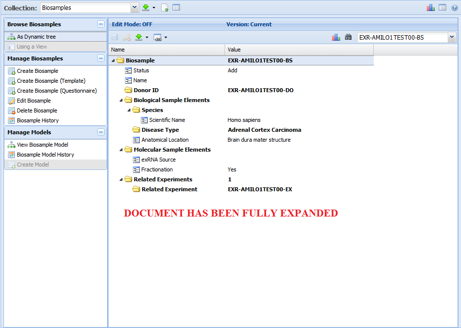
Now that you're viewing a metadata document, you might want to edit some properties, add new properties, etc.
The first thing you need to do is select the Edit option for the document, shown below:

In order to edit an existing property, all you need to do is double click the value for that property.
The possible values for a property depend upon that property's domain.
For example, if a property has a domain of string, you can pretty much write anything.
If a property has a domain of enum(a, b, c), you will only be able to pick a, b, or c.
Finally, if a property has a domain of bioPortal(...) or bioPortals(...), your value will be enforced by the ontologies listed in the domain.
To learn more about this feature, see the Dynamic Retrieval of Bioportal Ontology Terms section below.
You can view the domain for a given property by viewing the document model.
You can learn more about document models below.
Adding a new property is also easy.
Each property in a given metadata document is a child property (or subproperty) of another, parent property.
The only exception is the root property, which is the document identifier.
For example, in my biosample document, "Species" is a subproperty of "Biological Sample Elements", and "Scientific Name" is a subproperty of "Species".
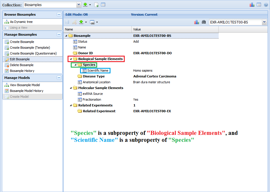
You can add a new subproperty by right clicking on a given property and then clicking the "Add" button:
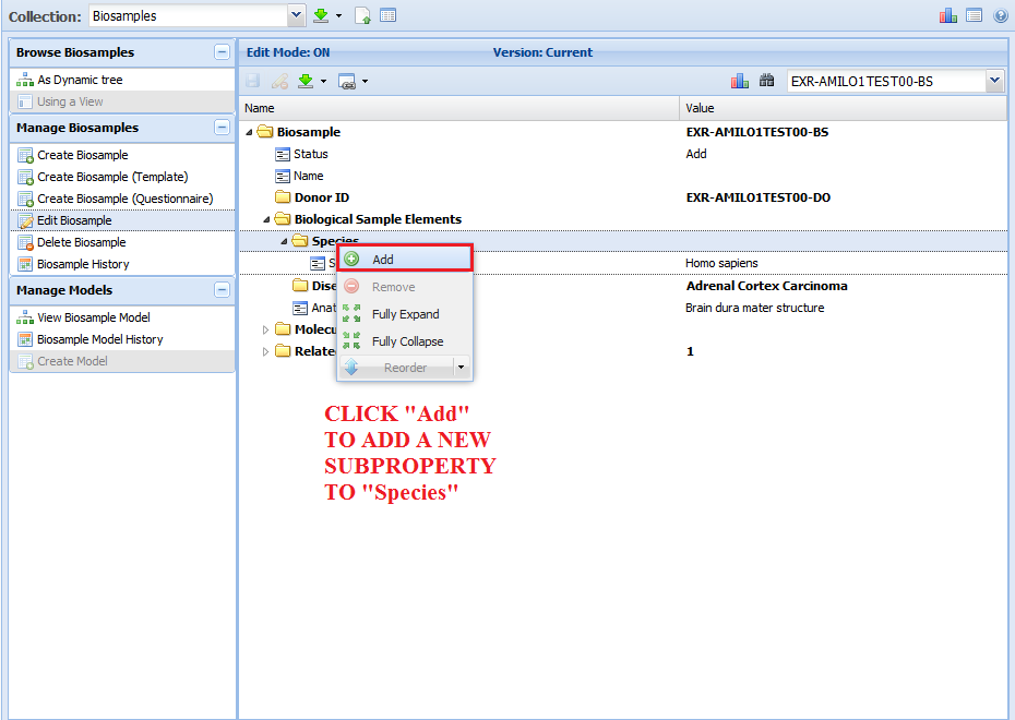
You are then presented with a list of valid subproperties that aren't already present in your document.
Choose the subproperty you want to add (I chose "Common Name") and then click "Update" to add the subproperty.

In order to see all of the different subproperties (so that you can properly build your document), you'll need to look at the document model.
Dynamic Retrieval of Bioportal Ontology Terms
While editing your document(s), you will most likely come across properties with a domain of "bioportalTerm" and/or "bioportalTerms".
These properties use a look ahead search field to dynamically retrieve ontology terms from Bioportal.
The search is performed on both the inputted term as well as synonyms for that term.
When entering a value for these properties, enter at least three characters to begin your search within the ontologies mentioned in the property's domain.
Once you see an appropriate value, select it and then confirm your choice by clicking the "Update" button.
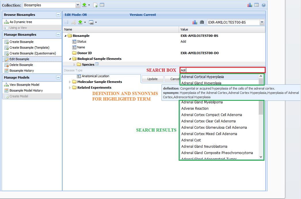
Once you're done editing your document, you can save it by clicking the "Save" button in the upper left corner of the GenboreeKB panel.
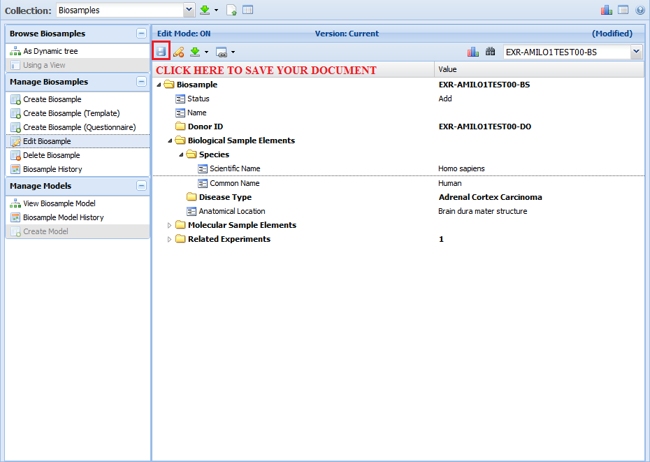
Before we finish saving your document, we will validate it to make sure that all required properties are present and all values are valid.
If you receive an error message when you try to save your document, follow the directions in that error message to correct your document.
Otherwise, if your document is valid, you will receive confirmation that the document was saved successfully.
There are three different ways to download docs in the GenboreeKB UI.
First, you can download an entire collection of docs at once. For example, if you want to download all of the docs in the Biosamples collection, you would use this option.
Second, you can download a single doc that you've opened in the UI. If you just want to grab one doc (maybe a single Biosample doc), you would use this option.
You can see both of these options in the image below:
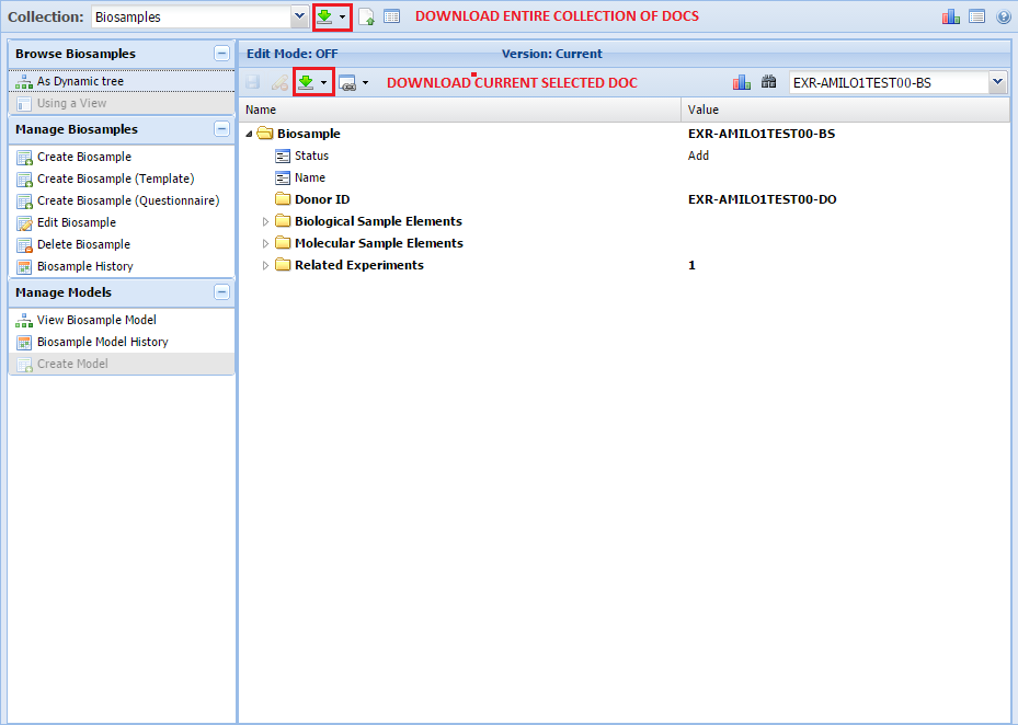
After you click either of the buttons, you'll have to select the format in which you'd like to receive your docs.
We recommend "Tabbed - Compact Property Names", since that's the format the FTP Pipeline accepts as valid input.
You could also pick the "Tabbed (Multi) - Compact Property Names" option if you are downloading an entire collection.
Currently, the FTP Pipeline only accepts this format for Biosample docs.
If you'd like to use this format for your own submission to the Atlas, downloading a collection in this format can be instructive for learning what the format looks like.
That way, you can construct your own Biosample submission in the proper way.
The third way to download docs is through the query feature highlighted above.
Simply perform a query and then click the green download icon in the toolbar to download all of the docs that are included in that query.
Each collection has its own document model.
This document model dictates the structure of the documents inside the collection.
Each document must conform to the rules set in the model.
For example, if the model states that a certain property is required, a document will not be valid unless it contains that property.
When we're building documents, the model is valuable because it tells us all of the different possible properties available for a document in the associated collection.
This will help us figure out which properties we need to add to our own document.
In order to see the document model associated with a given collection, click the "View Model" button as indicated below:
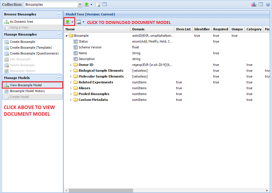
You can download a currently selected document model by clicking the green download icon highlighted in the above picture.
To learn more about what the different columns in the document model represent, you can check out the Data Model Schema page.
To see a full list of the different possible domains in GenboreeKB, click here.
To see a smaller list that contains explanations of some of the less intuitive domains, click here.
TABLE 1: List of Units supported by GenboreeKB
This table provides a list of all units that are currently supported by GenboreeKB.
| Unit Name |
Display Name |
Aliases |
Kind |
Scalar Value |
Definition |
| <gee> |
xG |
["gee", "standard-gravitation", "xG", "xg"] |
acceleration |
196133/20000 |
["<meter>"]/["<second>", "<second>"] |
| <katal> |
kat |
["kat", "katal"] |
activity |
1 |
["<mole>"]/["<second>"] |
| <unit> |
U |
["U", "enzUnit", "units", "unit"] |
activity |
1/60000000 |
["<mole>"]/["<second>"] |
| <degree> |
deg |
["deg", "degree", "degrees"] |
angle |
0.0174532925199433 |
["<radian>"]/["<1>"] |
| <grad> |
grad |
["grad", "gradian", "grads"] |
angle |
0.015707963267949 |
["<radian>"]/["<1>"] |
| <radian> |
rad |
["rad", "radian", "radians"] |
angle |
1 |
["<radian>"]/["<1>"] |
| <rotation> |
rotation |
["rotation"] |
angle |
6.28318530717959 |
["<radian>"]/["<1>"] |
| <rpm> |
rpm |
["rpm"] |
angular_velocity |
0.10471975511966 |
["<radian>"]/["<second>"] |
| <acre> |
acre |
["acre", "acres"] |
area |
316160658/78125 |
["<meter>", "<meter>"]/["<1>"] |
| <hectare> |
hectare |
["hectare"] |
area |
10000 |
["<meter>", "<meter>"]/["<1>"] |
| <sqft> |
sqft |
["sqft"] |
area |
145161/1562500 |
["<meter>", "<meter>"]/["<1>"] |
| <sqin> |
sqin |
["sqin"] |
area |
16129/25000000 |
["<meter>", "<meter>"]/["<1>"] |
| <farad> |
F |
["F", "farad", "farads"] |
capacitance |
1 |
["<ampere>", "<ampere>", "<second>", "<second>", "<second>", "<second>"]/["<kilogram>", "<meter>", "<meter>"] |
| <coulomb> |
C |
["C", "coulomb", "coulombs"] |
charge |
1 |
["<ampere>", "<second>"]/["<1>"] |
| <siemens> |
S |
["S", "siemens"] |
conductance |
1 |
["<ampere>", "<ampere>", "<second>", "<second>", "<second>"]/["<kilogram>", "<meter>", "<meter>"] |
| <base-pair> |
bp |
["bp", "base-pair"] |
counting |
1 |
["<each>"]/["<1>"] |
| <cell> |
cells |
["cells", "cell"] |
counting |
1 |
["<each>"]/["<1>"] |
| <count> |
count |
["count"] |
counting |
1 |
["<each>"]/["<1>"] |
| <dot> |
dot |
["dot", "dots"] |
counting |
1 |
["<each>"]/["<1>"] |
| <dozen> |
doz |
["doz", "dz", "dozen"] |
counting |
12 |
["<each>"]/["<1>"] |
| <each> |
each |
["each"] |
counting |
1 |
["<each>"]/["<1>"] |
| <gross> |
gr |
["gr", "gross"] |
counting |
144 |
["<each>"]/["<1>"] |
| <molecule> |
molecule |
["molecule", "molecules"] |
counting |
1 |
["<each>"]/["<1>"] |
| <nucleotide> |
nt |
["nt", "nucleotide"] |
counting |
1 |
["<each>"]/["<1>"] |
| <pixel> |
px |
["px", "pixel", "pixels"] |
counting |
1 |
["<each>"]/["<1>"] |
| <cents> |
cents |
["cents"] |
currency |
1/100 |
["<dollar>"]/["<1>"] |
| <dollar> |
USD |
["USD", "dollar"] |
currency |
1 |
["<dollar>"]/["<1>"] |
| <ampere> |
A |
["A", "ampere", "amperes", "amp", "amps"] |
current |
1 |
["<ampere>"]/["<1>"] |
| <btu> |
Btu |
["Btu", "btu", "Btus", "btus"] |
energy |
2320092679909671/2199023255552 |
["<kilogram>", "<meter>", "<meter>"]/["<second>", "<second>"] |
| <Calorie> |
Cal |
["Cal", "Calorie", "Calories"] |
energy |
4184.0 |
["<kilogram>", "<meter>", "<meter>"]/["<second>", "<second>"] |
| <calorie> |
cal |
["cal", "calorie", "calories"] |
energy |
4.184 |
["<kilogram>", "<meter>", "<meter>"]/["<second>", "<second>"] |
| <erg> |
erg |
["erg", "ergs"] |
energy |
1/10000000 |
["<kilogram>", "<meter>", "<meter>"]/["<second>", "<second>"] |
| <joule> |
J |
["J", "joule", "joules"] |
energy |
1 |
["<kilogram>", "<meter>", "<meter>"]/["<second>", "<second>"] |
| <therm> |
thm |
["thm", "therm", "therms", "Therm"] |
energy |
105505600.0 |
["<kilogram>", "<meter>", "<meter>"]/["<second>", "<second>"] |
| <dyne> |
dyn |
["dyn", "dyne"] |
force |
1/100000 |
["<kilogram>", "<meter>"]/["<second>", "<second>"] |
| <newton> |
N |
["N", "newton", "newtons"] |
force |
1 |
["<kilogram>", "<meter>"]/["<second>", "<second>"] |
| <poundal> |
pdl |
["pdl", "poundal", "poundals"] |
force |
17281869297/125000000000 |
["<kilogram>", "<meter>"]/["<second>", "<second>"] |
| <pound-force> |
lbf |
["lbf", "pound-force"] |
force |
8896443230521/2000000000000 |
["<kilogram>", "<meter>"]/["<second>", "<second>"] |
| <becquerel> |
Bq |
["Bq", "becquerel", "becquerels"] |
frequency |
1 |
["<1>"]/["<second>"] |
| <bpm> |
bpm |
["bpm"] |
frequency |
1/60 |
["<each>"]/["<second>"] |
| <cpm> |
cpm |
["cpm"] |
frequency |
1/60 |
["<each>"]/["<second>"] |
| <curie> |
Ci |
["Ci", "curie", "curies"] |
frequency |
37000000000.0 |
["<1>"]/["<second>"] |
| <dpm> |
dpm |
["dpm"] |
frequency |
1/60 |
["<each>"]/["<second>"] |
| <hertz> |
Hz |
["Hz", "hertz"] |
frequency |
1 |
["<1>"]/["<second>"] |
| <lux> |
lux |
["lux"] |
illuminance |
1 |
["<candela>", "<steradian>"]/["<meter>", "<meter>"] |
| <henry> |
H |
["H", "henry", "henries"] |
inductance |
1 |
["<kilogram>", "<meter>", "<meter>"]/["<ampere>", "<ampere>", "<second>", "<second>"] |
| <bit> |
b |
["b", "bit"] |
information |
1/8 |
["<byte>"]/["<1>"] |
| <byte> |
B |
["B", "byte", "bytes"] |
information |
1 |
["<byte>"]/["<1>"] |
| <angstrom> |
ang |
["ang", "angstrom", "angstroms"] |
length |
1/10000000000 |
["<meter>"]/["<1>"] |
| <AU> |
AU |
["AU", "astronomical-unit"] |
length |
149597870700 |
["<meter>"]/["<1>"] |
| <fathom> |
fathom |
["fathom", "fathoms"] |
length |
1143/625 |
["<meter>"]/["<1>"] |
| <foot> |
ft |
["ft", "foot", "feet", "'"] |
length |
381/1250 |
["<meter>"]/["<1>"] |
| <furlong> |
fur |
["fur", "furlong", "furlongs"] |
length |
25146/125 |
["<meter>"]/["<1>"] |
| <inch> |
in |
["in", "inch", "inches", "\""] |
length |
127/5000 |
["<meter>"]/["<1>"] |
| <league> |
league |
["league", "leagues"] |
length |
603504/125 |
["<meter>"]/["<1>"] |
| <light-minute> |
lmin |
["lmin", "light-minute"] |
length |
17987547480 |
["<meter>"]/["<1>"] |
| <light-second> |
ls |
["ls", "lsec", "light-second"] |
length |
299792458 |
["<meter>"]/["<1>"] |
| <light-year> |
ly |
["ly", "light-year"] |
length |
9460528412464108 |
["<meter>"]/["<1>"] |
| <meter> |
m |
["m", "meter", "meters", "metre", "metres"] |
length |
1 |
["<meter>"]/["<1>"] |
| <mile> |
mi |
["mi", "mile", "miles"] |
length |
201168/125 |
["<meter>"]/["<1>"] |
| <mil> |
mil |
["mil", "mils"] |
length |
127/5000000 |
["<meter>"]/["<1>"] |
| <naut-league> |
nleague |
["nleague", "nleagues", "naut-league"] |
length |
5556 |
["<meter>"]/["<1>"] |
| <naut-mile> |
nmi |
["nmi", "M", "NM", "naut-mile"] |
length |
1852 |
["<meter>"]/["<1>"] |
| <parsec> |
pc |
["pc", "parsec", "parsecs"] |
length |
3.08568025088532e+16 |
["<meter>"]/["<1>"] |
| <pica> |
P |
["P", "pica", "picas"] |
length |
127/30000 |
["<meter>"]/["<1>"] |
| <point> |
point |
["point", "points"] |
length |
127/360000 |
["<meter>"]/["<1>"] |
| <redshift> |
z |
["z", "red-shift", "redshift"] |
length |
130277299999999992243683328 |
["<meter>"]/["<1>"] |
| <rod> |
rd |
["rd", "rod", "rods"] |
length |
12573/2500 |
["<meter>"]/["<1>"] |
| <survey-foot> |
sft |
["sft", "sfoot", "sfeet", "survey-foot"] |
length |
1200/3937 |
["<meter>"]/["<1>"] |
| <yard> |
yd |
["yd", "yard", "yards"] |
length |
1143/1250 |
["<meter>"]/["<1>"] |
| <decibel> |
dB |
["dB", "decibel", "decibels"] |
logarithmic |
1 |
["<decibel>"]/["<1>"] |
| <candela> |
cd |
["cd", "candela"] |
luminosity |
1 |
["<candela>"]/["<1>"] |
| <lumen> |
lm |
["lm", "lumen"] |
luminous_power |
1 |
["<candela>", "<steradian>"]/["<1>"] |
| <gauss> |
G |
["G", "gauss"] |
magnetism |
1/10000 |
["<kilogram>"]/["<ampere>", "<second>", "<second>"] |
| <maxwell> |
Mx |
["Mx", "maxwell", "maxwells"] |
magnetism |
1/100000000 |
["<kilogram>", "<meter>", "<meter>"]/["<ampere>", "<second>", "<second>"] |
| <oersted> |
Oe |
["Oe", "oersted", "oersteds"] |
magnetism |
79.5774715459477 |
["<ampere>"]/["<meter>"] |
| <tesla> |
T |
["T", "tesla", "teslas"] |
magnetism |
1 |
["<kilogram>"]/["<ampere>", "<second>", "<second>"] |
| <weber> |
Wb |
["Wb", "weber", "webers"] |
magnetism |
1 |
["<kilogram>", "<meter>", "<meter>"]/["<ampere>", "<second>", "<second>"] |
| <AMU> |
u |
["u", "AMU", "amu"] |
mass |
1/602214128999999968641024 |
["<kilogram>"]/["<1>"] |
| <carat> |
ct |
["ct", "carat", "carats"] |
mass |
1/5000 |
["<kilogram>"]/["<1>"] |
| <dalton> |
Da |
["Da", "dalton", "daltons"] |
mass |
1/602214128999999968641024 |
["<kilogram>"]/["<1>"] |
| <gram> |
g |
["g", "gram", "grams", "gramme", "grammes"] |
mass |
1/1000 |
["<kilogram>"]/["<1>"] |
| <kilogram> |
kg |
["kg", "kilogram", "kilograms"] |
mass |
1 |
["<kilogram>"]/["<1>"] |
| <metric-ton> |
tonne |
["tonne", "metric-ton"] |
mass |
1000 |
["<kilogram>"]/["<1>"] |
| <ounce> |
oz |
["oz", "ounce", "ounces"] |
mass |
45359237/1600000000 |
["<kilogram>"]/["<1>"] |
| <pound> |
lbs |
["lbs", "lb", "lbm", "pound-mass", "pound", "pounds", "#"] |
mass |
45359237/100000000 |
["<kilogram>"]/["<1>"] |
| <short-ton> |
tn |
["tn", "ton", "tons", "short-tons", "short-ton"] |
mass |
45359237/50000 |
["<kilogram>"]/["<1>"] |
| <slug> |
slug |
["slug", "slugs"] |
mass |
8896443230521/609600000000 |
["<kilogram>"]/["<1>"] |
| <molar> |
M |
["M", "molar"] |
molar_concentration |
1000 |
["<mole>"]/["<meter>", "<meter>", "<meter>"] |
| <volt> |
V |
["V", "volt", "volts"] |
potential |
1 |
["<kilogram>", "<meter>", "<meter>"]/["<ampere>", "<second>", "<second>", "<second>"] |
| <horsepower> |
hp |
["hp", "horsepower"] |
power |
37284993579113511/50000000000000 |
["<kilogram>", "<meter>", "<meter>"]/["<second>", "<second>", "<second>"] |
| <watt> |
W |
["W", "Watt", "watt", "watts"] |
power |
1 |
["<kilogram>", "<meter>", "<meter>"]/["<second>", "<second>", "<second>"] |
| <atm> |
atm |
["atm", "ATM", "atmosphere", "atmospheres"] |
pressure |
101325 |
["<kilogram>"]/["<second>", "<second>", "<meter>"] |
| <bar> |
bar |
["bar", "bars"] |
pressure |
100000.0 |
["<kilogram>"]/["<second>", "<second>", "<meter>"] |
| <cmh2o> |
cmH2O |
["cmH2O", "cmh2o", "cmAq"] |
pressure |
196133/2000 |
["<kilogram>"]/["<second>", "<second>", "<meter>"] |
| <inh2o> |
inH2O |
["inH2O", "inh2o", "inAq"] |
pressure |
24908891/100000 |
["<kilogram>"]/["<second>", "<second>", "<meter>"] |
| <inHg> |
inHg |
["inHg"] |
pressure |
190636732734642608180389/56294995342131200000 |
["<kilogram>"]/["<second>", "<second>", "<meter>"] |
| <mmHg> |
mmHg |
["mmHg"] |
pressure |
1501076635705847308507/11258999068426240000 |
["<kilogram>"]/["<second>", "<second>", "<meter>"] |
| <pascal> |
Pa |
["Pa", "pascal", "pascals"] |
pressure |
1 |
["<kilogram>"]/["<meter>", "<second>", "<second>"] |
| <psi> |
psi |
["psi"] |
pressure |
8896443230521/1290320000 |
["<kilogram>"]/["<second>", "<second>", "<meter>"] |
| <torr> |
Torr |
["Torr", "torr"] |
pressure |
20265/152 |
["<kilogram>"]/["<second>", "<second>", "<meter>"] |
| <gray> |
Gy |
["Gy", "gray", "grays"] |
radiation |
1 |
["<meter>", "<meter>"]/["<second>", "<second>"] |
| <sievert> |
Sv |
["Sv", "sievert", "sieverts"] |
radiation |
1 |
["<meter>", "<meter>"]/["<second>", "<second>"] |
| <roentgen> |
R |
["R", "roentgen"] |
radiation_exposure |
0.000258 |
["<ampere>", "<second>"]/["<kilogram>"] |
| <ohm> |
Ohm |
["Ohm", "ohm", "ohms"] |
resistance |
1 |
["<kilogram>", "<meter>", "<meter>"]/["<ampere>", "<ampere>", "<second>", "<second>", "<second>"] |
| <steradian> |
sr |
["sr", "steradian", "steradians"] |
solid_angle |
1 |
["<steradian>"]/["<1>"] |
| <fps> |
fps |
["fps"] |
speed |
381/1250 |
["<meter>"]/["<second>"] |
| <knot> |
kt |
["kt", "kn", "kts", "knot", "knots"] |
speed |
463/900 |
["<meter>"]/["<second>"] |
| <kph> |
kph |
["kph"] |
speed |
0.277777777777778 |
["<meter>"]/["<second>"] |
| <mph> |
mph |
["mph"] |
speed |
1397/3125 |
["<meter>"]/["<second>"] |
| <mole> |
mol |
["mol", "mole"] |
substance |
1 |
["<mole>"]/["<1>"] |
| <celsius> |
degC |
["degC", "celsius", "centigrade"] |
temperature |
1 |
["<kelvin>"]/["<1>"] |
| <fahrenheit> |
degF |
["degF", "fahrenheit"] |
temperature |
2501999792983609/4503599627370496 |
["<kelvin>"]/["<1>"] |
| <kelvin> |
degK |
["degK", "kelvin"] |
temperature |
1 |
["<kelvin>"]/["<1>"] |
| <rankine> |
degR |
["degR", "rankine"] |
temperature |
2501999792983609/4503599627370496 |
["<kelvin>"]/["<1>"] |
| <tempC> |
tempC |
["tempC"] |
temperature |
1 |
["<tempK>"]/["<1>"] |
| <tempF> |
tempF |
["tempF"] |
temperature |
2501999792983609/4503599627370496 |
["<tempK>"]/["<1>"] |
| <tempK> |
tempK |
["tempK"] |
temperature |
1 |
["<tempK>"]/["<1>"] |
| <tempR> |
tempR |
["tempR"] |
temperature |
255.927777777778 |
["<tempK>"]/["<1>"] |
| <century> |
century |
["century", "centuries"] |
time |
3155692600 |
["<second>"]/["<1>"] |
| <day> |
d |
["d", "day", "days"] |
time |
86400 |
["<second>"]/["<1>"] |
| <decade> |
decade |
["decade", "decades"] |
time |
315569260 |
["<second>"]/["<1>"] |
| <fortnight> |
fortnight |
["fortnight", "fortnights"] |
time |
1209600 |
["<second>"]/["<1>"] |
| <hour> |
h |
["h", "hr", "hrs", "hour", "hours"] |
time |
3600 |
["<second>"]/["<1>"] |
| <minute> |
min |
["min", "minute", "minutes"] |
time |
60 |
["<second>"]/["<1>"] |
| <month> |
Month |
["month", "mon", "months", "mons", "mo"] |
time |
2629743.83333333 |
["<second>"]/["<1>"] |
| <second> |
s |
["s", "sec", "second", "seconds"] |
time |
1 |
["<second>"]/["<1>"] |
| <week> |
wk |
["wk", "week", "weeks"] |
time |
604800 |
["<second>"]/["<1>"] |
| <year> |
y |
["y", "yr", "year", "years", "annum"] |
time |
31556926 |
["<second>"]/["<1>"] |
| <percent> |
% |
["%", "percent"] |
unitless |
1/100 |
|
| <ppb> |
ppb |
["ppb"] |
unitless |
1/1000000000 |
|
| <ppm> |
ppm |
["ppm"] |
unitless |
1/1000000 |
|
| <poise> |
P |
["P", "poise"] |
viscosity |
1/10 |
["<kilogram>"]/["<second>", "<meter>"] |
| <stokes> |
St |
["St", "stokes"] |
viscosity |
1/10000 |
["<meter>", "<meter>"]/["<second>"] |
| <cup> |
cu |
["cu", "cup", "cups"] |
volume |
473176473/2000000000000 |
["<meter>", "<meter>", "<meter>"]/["<1>"] |
| <fluid-ounce> |
floz |
["floz", "fluid-ounce", "fluid-ounces"] |
volume |
473176473/16000000000000 |
["<meter>", "<meter>", "<meter>"]/["<1>"] |
| <gallon> |
gal |
["gal", "gallon", "gallons"] |
volume |
473176473/125000000000 |
["<meter>", "<meter>", "<meter>"]/["<1>"] |
| <liter> |
l |
["l", "L", "liter", "liters", "litre", "litres"] |
volume |
1/1000 |
["<meter>", "<meter>", "<meter>"]/["<1>"] |
| <pint> |
pt |
["pt", "pint", "pints"] |
volume |
473176473/1000000000000 |
["<meter>", "<meter>", "<meter>"]/["<1>"] |
| <quart> |
qt |
["qt", "quart", "quarts"] |
volume |
473176473/500000000000 |
["<meter>", "<meter>", "<meter>"]/["<1>"] |
| <tablespoon> |
tbs |
["tbs", "tbsp", "tablespoon", "tablespoons"] |
volume |
473176473/32000000000000 |
["<meter>", "<meter>", "<meter>"]/["<1>"] |
| <teaspoon> |
tsp |
["tsp", "teaspoon", "teaspoons"] |
volume |
157725491/32000000000000 |
["<meter>", "<meter>", "<meter>"]/["<1>"] |
| <cfm> |
cfm |
["cfm", "CFM", "CFPM"] |
volumetric_flow |
18435447/39062500000 |
["<meter>", "<meter>", "<meter>"]/["<second>"] |
| <dpi> |
dpi |
["dpi"] |
wavenumber |
5000/127 |
["<each>"]/["<meter>"] |
| <ppi> |
ppi |
["ppi"] |
wavenumber |
5000/127 |
["<each>"]/["<meter>"] |
TABLE 2: Scales of Units
Below is a list of acceptable prefixes to the units provided in Table 1.
You can use a combination of the prefix from Table 2 and the actual unit name from Table 1
when you define units for measurement domain properties.
EXAMPLE:
- microgram can be used if your domain definition is ng
| Prefix Name |
Display Name |
Aliases |
Kind |
Scalar Value |
| <1> |
1 |
["1"] |
prefix |
1 |
| <atto> |
a |
["a", "Atto", "atto"] |
prefix |
1/1000000000000000000 |
| <centi> |
c |
["c", "Centi", "centi"] |
prefix |
1/100 |
| <deca> |
da |
["da", "Deca", "deca", "deka"] |
prefix |
10.0 |
| <deci> |
d |
["d", "Deci", "deci"] |
prefix |
1/10 |
| <exa> |
E |
["E", "Exa", "exa"] |
prefix |
1.0e+18 |
| <exi> |
Ei |
["Ei", "Exi", "exi"] |
prefix |
1152921504606846976 |
| <femto> |
f |
["f", "Femto", "femto"] |
prefix |
1/1000000000000000 |
| <gibi> |
Gi |
["Gi", "Gibi", "gibi"] |
prefix |
1073741824 |
| <giga> |
G |
["G", "Giga", "giga"] |
prefix |
1000000000.0 |
| <googol> |
googol |
["googol"] |
prefix |
1.0e+100 |
| <hecto> |
h |
["h", "Hecto", "hecto"] |
prefix |
100.0 |
| <kibi> |
Ki |
["Ki", "Kibi", "kibi"] |
prefix |
1024 |
| <kilo> |
k |
["k", "kilo"] |
prefix |
1000.0 |
| <mebi> |
Mi |
["Mi", "Mebi", "mebi"] |
prefix |
1048576 |
| <mega> |
M |
["M", "Mega", "mega"] |
prefix |
1000000.0 |
| <micro> |
u |
["u", "Micro", "micro", "mc"] |
prefix |
1/1000000 |
| <milli> |
m |
["m", "Milli", "milli"] |
prefix |
1/1000 |
| <nano> |
n |
["n", "Nano", "nano"] |
prefix |
1/1000000000 |
| <pebi> |
Pi |
["Pi", "Pebi", "pebi"] |
prefix |
1125899906842624 |
| <peta> |
P |
["P", "Peta", "peta"] |
prefix |
1.0e+15 |
| <pico> |
p |
["p", "Pico", "pico"] |
prefix |
1/1000000000000 |
| <tebi> |
Ti |
["Ti", "Tebi", "tebi"] |
prefix |
1099511627776 |
| <tera> |
T |
["T", "Tera", "tera"] |
prefix |
1000000000000.0 |
| <yebi> |
Yi |
["Yi", "Yebi", "yebi"] |
prefix |
1208925819614629174706176 |
| <yocto> |
y |
["y", "Yocto", "yocto"] |
prefix |
1/999999999999999983222784 |
| <yotta> |
Y |
["Y", "Yotta", "yotta"] |
prefix |
1.0e+24 |
| <zebi> |
Zi |
["Zi", "Zebi", "zebi"] |
prefix |
1180591620717411303424 |
| <zepto> |
z |
["z", "Zepto", "zepto"] |
prefix |
1/1000000000000000000000 |
| <zetta> |
Z |
["Z", "Zetta", "zetta"] |
prefix |
1.0e+21 |
Overview
Step-by-step Instructions to Use GenboreeKB
In order to see TEMPLATES and EXAMPLES for the various collections you'll be browsing, refer to exRNA Metadata Standards.
Login
- Log in to GenboreeKB using your Genboree user name and password.
- If you are a member of the ERCC, you will be able to access both the public Atlas and private, ERCC-only Atlas.
- In order to get access to the private Atlas KB, you will need to contact "Emily after you login for the first time.
- One of us will grant you permission to see the private Atlas KB in your Projects page.
- Non-ERCC members can only access the public Atlas.
GenboreeKB Basics


Add Sub-properties


Saving Document

Search and Browse Existing Documents


Edit Existing Documents


Dynamic Retrieval of Bioportal Ontology Terms

Bulk Upload of Docs

Download entire collection or a single document

Data Models
View Models


Given below are the instructions to ensure your metadata file is formatted
and opened correctly in Microsoft Excel.
- Open Microsoft Excel.
- Click on File
>> Open, then navigate to the folder in your computer that has the saved metadata file.
- Select the metadata file (with .tsv extension)
- Choose the file type as "Delimited" and click Next.
- Check the box next to Tab Delimiter and click Next.
- IMPORTANT STEP: Select the radio button next to Text under Column data format and click Finish.
IMPORTANT: Make sure that you open the file through File >> Open in Excel as opposed to right-clicking the file and then clicking open with Excel. The latter method may bypass the text import wizard and result in issues with your metadata file.
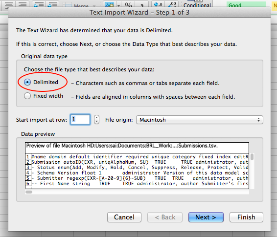
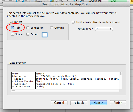
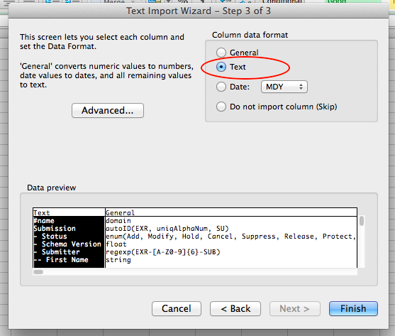
Microsoft Excel in Windows
Select "Save As" from the menubar.
Navigate to the folder where you would like to save your metadata document.
Provide a file name for your document. Remember, file names end with .metadata.tsv.
Select the option "Text (Tab delimited)" from the pull down menu for "Save as type" and press OK.
Microsoft Excel in Mac
To save your metadata documents as a properly formatted tab-separated value file, click "Save" and
select the option to save as "Windows Formatted Text".
This option saves the file as a tab-separated value file without any special characters.
LibreOffice Calc
Select "Save As", choose "All Format", and then choose "Test CSV (.csv)".
You will see a dialog box titled "Export Text File".
Select {Tab} from the pull down menu for "Field delimiter" and select OK.
Your document will be saved as a tab-delimited text file.
Sanity Check the TSV file
To ensure there are no special characters in your metadata document after following the above mentioned
methods to save your file, open the document in any text editor like
- Notepad (Windows),
- gedit (Ubuntu/Linux),
- TextEdit (Mac) or
- command line editors like vim, nano, etc. in the Terminal (Linux/Unix/Mac OSX).
Check if the document is properly formatted, i.e. columns are separated by a tab character and
the document does not have any characters like ^M, etc.
Given below are the instructions to ensure your metadata template document is formatted
and opened correctly in Microsoft Excel.
- Open Microsoft Excel.
- Click on File
>> Open, then navigate to the folder in your computer that has the saved document template.
- Select the document template file (with .tsv extension)
- Choose the file type as "Delimited" and click Next.
- Check the box next to Tab Delimiter and click Next.
- IMPORTANT STEP: Select the radio button next to Text under Column data format and click Finish.
Microsoft Excel in Windows
Select "Save As" from the menubar.
Navigate to the folder where you would like to save your metadata document.
Provide a file name for your document. Remember, file names end with .metadata.tsv.
Select the option "Text (Tab delimited)" from the pull down menu for "Save as type" and press OK.
Microsoft Excel in Mac
To save your metadata documents as a properly formatted tab-separated value file, click "Save" and
select the option to save as "Windows Formatted Text".
This option saves the file as a tab-separated value file without any special characters.
LibreOffice Calc
Select "Save As", choose "All Format", and then choose "Test CSV (.csv)".
You will see a dialog box titled "Export Text File".
Select {Tab} from the pull down menu for "Field delimiter" and select OK.
Your document will be saved as a tab-delimited text file.
Sanity Check the TSV file
To ensure there are no special characters in your metadata document after following the above mentioned
methods to save your file, open the document in any text editor like
- Notepad (Windows),
- gedit (Ubuntu/Linux),
- TextEdit (Mac) or
- command line editors like vim, nano, etc. in the Terminal (Linux/Unix/Mac OSX).
Check if the document is properly formatted, i.e. columns are separated by a tab character and
the document does not have any characters like ^M, etc.
- First, download the template linked here.
- After you've opened the template, you will provide values in the value column.
- At this point, if you haven't created a metadata file before, you should read through the Understanding the Nested Tabbed Format page to better understand how your file is formatted.
- You are only required to provide values for those properties which have TRUE in the required column.
- Even if a property has TRUE in the required column, if its parent property does NOT have TRUE in the required column, then you are not required to fill in the (sub) property.
- If you want to see a completed Analyses metadata file, you can download one here.
- WE HIGHLY RECOMMEND YOU DOWNLOAD THE EXAMPLE, AS IT WILL MAKE UNDERSTANDING THE DIRECTIONS BELOW MUCH EASIER!
- Here are some specific instructions for filling out an Analyses metadata file:
- For the Analysis property, the value will look something like this: EXR-AMILO1GASTCANC-AN.
- The ID will always start with EXR- (this stands for exRNA).
- Next, I wrote AMILO1 because my PI is Aleksandar MILOsavljevic (AMILO). The 1 indicates that he is the first PI with this particular ID. If you're not sure about your PI ID, feel free to contact Emily.
- Third, I wrote GASTCANC to give some information about my study. Here, my study is studying gastric cancer, so I wrote GASTCANC.
- Finally, the value ends with -AN to indicate that the file is a Analyses file.
- For the - Status property, you can write either "Add" or "Protect".
- Write "Add" if you want to add your files to the public Atlas immediately.
- Write "Protect" if you want to keep your files in the consortium-only Atlas until the embargo period ends on your submission.
- For the - Date of Analysis property, you should write the date you're submitting your files to the DCC.
- Write the date in the format YYYY/MM/DD. For example, if I was submitting my files on September 21st, 2017, I would write 2017/09/21.
- For the * Conditions Associated with Analysis property, you don't need to write anything, but don't delete it!
- Underneath the * Conditions Associated with Analysis property, you should write one *- Condition property for each condition mentioned in your Biosamples file.
- For example, if I had three different conditions ("Healthy Control", "glioblastoma multiforme", and "Alzheimer's Disease") mentioned in my Biosamples file, I would list these conditions like the following:
- *- Condition Healthy Control
- *- Condition glioblastoma multiforme
- *- Condition Alzheimer's Disease
- For the - Data Analysis Level property, you don't need to write anything, but don't delete it!
- For the -- Type property, you should write "qPCR Data Analysis".
- For the --- qPCR Data Analysis Level property, you don't need to write anything, but don't delete it!
- You should then fill out all relevant subproperties underneath the --- qPCR Data Analysis Level property.
- In particular, you should fill out the ---* Biosamples property and its subproperties.
- For the ---* Biosamples property, you don't need to write anything, but don't delete it!
- Underneath the ---* Biosamples property, you should write one ---*- Biosample ID property for each biosample in your submission. The value for each line should be a different biosample in your submission.
- Underneath each ---*- Biosample ID property, you should write one ---*-- DocURL property. The value for each line should be "coll/Biosamples/doc/" and then your biosample ID. For example, you could write "coll/Biosamples/doc/EXR-AMILO1GASTCANC1-BS" if that was a valid biosample ID for your submission.
- Underneath each ---*- Biosample ID property, you should write one ---*-- qPCR Target Doc ID property. The value for each line should be the qPCR Target ID associated with the relevant biosample ID. For example, if my EXR-AMILO1GASTCANC1-BS biosample had an associated qPCR Targets ID of EXR-AMILO1GASTCANC1-QT, I would write "EXR-AMILO1GASTCANC1-QT".
- Underneath each ---*-- qPCR Target Doc ID property, you should write one ---*--- DocURL property. The value for each line should be "/coll/qPCR%20Targets/doc/" and then your qPCR Targets ID. For example, you could write "coll/qPCR%20Targets/doc/EXR-AMILO1GASTCANC1-QT".
- If you're confused by the directions above related to the ---* Biosamples property and its subproperties, you should look at the COMPLETED ANALYSES EXAMPLE FILE.
- If you didn't fill out a value for a property, then please delete the row containing that property from your file. Make sure that you actually remove the row entirely and don't leave a blank row!
However, if the domain for the property is [valueless] and you filled out values for any subproperties, then don't delete the row.
- Finally, save your metadata file in tab-delimited format with a file name that ends in .metadata.tsv.
- I recommend you name your metadata file after the value given for your Analysis property.
- For example, I would name my metadata file EXR-AMILO1GASTCANC-AN.metadata.tsv.
- If you need help saving your metadata file, we have instructions available here.
- First, download the template linked here.
- After you've opened the template, you will provide values in the value column.
- Note that your submission will likely have multiple biosamples associated with it.
- It's easy to handle multiple biosamples - just create a new value column for each additional biosample.
- For example, if I had 20 biosamples associated with my submission, I would create 19 additional value columns to the right of the one currently present in the template.
- At this point, if you haven't created a metadata file before, you should read through the Understanding the Nested Tabbed Format page to better understand how your file is formatted.
- You are only required to provide values for those properties which have TRUE in the required column.
- Even if a property has TRUE in the required column, if its parent property does NOT have TRUE in the required column, then you are not required to fill in the (sub) property.
- If you want to see a completed Biosamples metadata file, you can download one here.
Here are some specific instructions for filling out a Biosamples metadata file:
- For the Biosample property, each value will look something like this: EXR-AMILO1GASTCANC1-BS.
- The ID will always start with EXR- (this stands for exRNA).
- Next, I wrote AMILO1 because my PI is Aleksandar MILOsavljevic (AMILO). The 1 indicates that he is the first PI with this particular ID. If you're not sure about your PI ID, feel free to contact exRNA Team.
- Third, I wrote GASTCANC1 to give some information about my biosample. Here, my biosample is connected with a gastric cancer study, so I wrote GASTCANC and then 1 (because we're discussing the first value currently).
- Finally, the value ends with -BS to indicate that the file is a Biosamples file.
- If I had a second biosample, I would write something like EXR-AMILO1GASTCANC2-BS in my second value column.
- Make sure each biosample property is unique
- For the - Status property, you can write either "Add" or "Protect".
- Write "Add" if you want to add your files to the public Atlas immediately.
- Write "Protect" if you want to keep your files in the consortium-only Atlas until the embargo period ends on your submission.
- For the - Name property, you should write a name for your biosample that conveys some important information about that sample.
- No two biosamples should have the same name within your submission.
- For the - Donor ID property, you should write the ID for the donor associated with the biosample.
- For example, if the donor EXR-AMILO1GASTCANC1-DO is associated with the current biosample, I would write EXR-AMILO1GASTCANC1-DO.
- You should also fill in the *-- DocURL subproperty with the same ID but in the following format: coll/Donors/doc/ and then your ID.
- I would put coll/Donors/doc/EXR-AMILO1GASTCANC1-DO.
- The same Donor ID can be used for multiple biosamples if they are coming from the same Donor.
- Example 1: A donor has donated both blood and skin biosamples, each would get the same Donor ID but get an unique Biosample ID.
- Example 2: In a time course experiment, the same sample collected at two time points would be represented by the same Donor ID, but each time point would get an unique Biosample ID
- You don't need to write anything for the - Biological Sample Elements property, but don't delete it from your file!
- You don't need to write anything for the -- Species property, but don't delete it from your file!
- For the --- Scientific Name property, you should write Homo sapiens or Mus musculus.
- For the --- Common Name property, you should write Human or Mouse.
- For the -- Disease Type property, your value will be enforced by ontologies.
- Here is a list of previously used values for this property:
- glioblastoma multiforme, colorectal cancer, Ulcerative Colitis, Healthy Control, Healthy Subject, Gastric Cancer Pathologic TNM Finding v7, Cardiovascular Disorder, Alzheimer's Disease, Subarachnoid Hemorrhage, Parkinson's Disease, Intraventricular Brain Hemorrhage, Systemic Lupus Erythematosus, Chronic Maternal Hypertension with Superimposed Preeclampsia, severe pre-eclampsia, pre-eclampsia, Fetus Small for Gestational Age, HELLP Syndrome, Nephrotic Syndrome, liver disease, Colon Carcinoma, Prostate Carcinoma, Pancreatic Carcinoma
- If your disease type is not listed above, then follow these steps:
- Visit the GenboreeKB UI template for Donors (you will need to log into your GenboreeKB account if not already logged in) here.
- Double click the pencil icon next to the Disease Type property.
- Begin typing the name of your disease type. After you type at least 3 characters, our look-ahead search will attempt to find matching terms in the ontology.
- Any term that pops up will be a valid value for your property. You can copy paste it into your Biosamples metadata file.
- If you still can't find an appropriate term for your disease type, feel free to contact the exRNA Team .
- For the -- Anatomical Location property, your value will be enforced by ontologies.
- Here is a list of previously used values for this property:
- Cellular analyte, Entire cardiovascular system, Entire oral cavity, Colon part, Structure of nervous tissue, Entire brain, Brain ventricle structure, Entire body system, High density lipoprotein, Urinary system structure, Entire bile duct
- If your anatomical location is not listed above, then follow the steps above for Disease Type to find a valid value.
Just double click the pencil icon next to Anatomical Location instead of Disease Type.
- If your biosample is biofluid-based, then you will want to leave the -- Biological Fluid property in your metadata file - you don't need to fill in a value, but don't delete it!
- You will then want to fill in a value for the --- Biofluid Name property. Your value will be enforced by ontologies.
- Here is a list of previously used values for this property:
- Culture Media, Conditioned, Plasma, Saliva, Cerebrospinal fluid, Serum, Urine, Bile
- If your anatomical location is not listed above, then follow the steps above for Disease Type to find a valid value.
Just double click the pencil icon next to Biofluid Name instead of Disease Type.
- If your biosample is cell culture supernatant-based, then you will want to leave the -- Cell Culture Supernatant property in your metadata file - you don't need to fill in a value, but don't delete it!
- You will then want to fill in values for the --- Source, ---- Type, --- Tissue, and ---- Tissue Type properties. Your values will be enforced by ontologies.
- Here is a list of previously used values for --- Source:
- Tumor Tissue, Human Cell Line
- Here is a list of previously used values for ---- Type:
- cell culture, colorectal cancer cell
- Here is a list of previously used values for --- Tissue:
- Here is a list of previously used values for ---- Tissue Type:
- Tumor tissue sample, frozen specimen
- If your values for any of the required properties are not listed above, then follow the steps above for Disease Type to find a valid value.
Just double click the pencil icon next to the property name (Source, Type, Tissue, Tissue Type) instead of Disease Type.
- You don't need to write anything for the - Molecular Sample Elements property, but don't delete it from your file!
- For the -- exRNA Source property, you should put one of the following values:
- extracellular exosome, extracellular vesicle, HDL-containing protein-lipid-RNA complex, total cell-free biofluid RNA, ribonucleoprotein complex, protein-lipid-RNA complex, LDL-containing protein-lipid-RNA complex, apoptotic body
- For the -- Fractionation property, you should put Yes or No.
- Finally, you should put the value 1 for the * Related Experiments property.
- For the *- Related Experiment subproperty, write the Experiments ID for the experiment associated with the current biosample.
- I might put EXR-AMILO1GASTCANC1-EX, for example.
- For the *-- DocURL subproperty, write the same ID but in the following format: coll/Experiments/doc/ and then your ID.
- I would put coll/Experiments/doc/EXR-AMILO1GASTCANC1-EX.
- If you didn't fill out a value for a property, then please delete the row containing that property from your file. Make sure that you actually remove the row entirely and don't leave a blank row!
However, if the domain for the property is [valueless] and you filled out values for any subproperties, then don't delete the row.
- Finally, save your metadata file in tab-delimited format with a file name that ends in .metadata.tsv.
- I recommend you name your metadata file after the value given for your Biosample property (excluding the identifying number at the end if you have multiple documents).
- For example, I would name my metadata file EXR-AMILO1GASTCANC-BS.metadata.tsv.
- If you need help saving your metadata file, we have instructions available here.
Prepare Your Data Archive
- Your data files should all be FASTQ / SRA single-end sequencing read files.
- It is acceptable for individual FASTQ / SRA files to be compressed.
- If you wish to include a spike-in FASTA file, that file should also be included in your data archive.
Step 1. Gather All of Your Data Files in the Same Directory
- Move all of your data files (FASTQ / SRA files) into the same directory.
- Optionally, you can also include a FASTA file with spike-in sequences for your samples.
- You cannot include multiple spike-in sequence files. Only one FASTA file is allowed.
Step 2. Compress Data Files into One Archive
- Place all data files into a single archive.
- The archive must be .tar.gz or .zip format.
- The data archive's file name must end in _data.
- For example, "samples_data.zip" would be valid. So would "exRNA_data.tar.gz".
- If you need help creating an archive, please visit the Creating an Archive page.
- IMPORTANT: If you are creating your archive on a Mac, please create a .tar.gz and not a .zip.
We have run into some issues with decompressing large zip archives that were created using the Mac archiving software.
Summary
- Gather all of your data files in the same directory (including spike-in file, if necessary)
- Compress data files into a single archive
- First, download the template linked here.
- After you've opened the template, you will provide values in the value column.
- Note that your submission will likely have multiple donors associated with it.
- It's easy to handle multiple donors - just create a new value column for each additional donor.
- For example, if I had 3 donors associated with my submission, I would create two additional value columns to the right of the one currently present in the template.
- At this point, if you haven't created a metadata file before, you should read through the Understanding the Nested Tabbed Format page to better understand how your file is formatted.
- You are only required to provide values for those properties which have TRUE in the required column.
- Even if a property has TRUE in the required column, if its parent property does NOT have TRUE in the required column, then you are not required to fill in the (sub) property.
- If you want to see a completed Donors metadata file, you can download one here.
Here are some specific instructions for filling out a Donors metadata file:
- For the Donor property, each value will look something like this: EXR-AMILO1GASTCANC1-DO.
- The ID will always start with EXR- (this stands for exRNA).
- Next, I wrote AMILO1 because my PI is Aleksandar MILOsavljevic (AMILO). The 1 indicates that he is the first PI with this particular ID. If you're not sure about your PI ID, feel free to contact exRNA Team .
- Third, I wrote GASTCANC1 to give some information about my donor. Here, my donor is connected with a gastric cancer study, so I wrote GASTCANC and then 1 (because we're discussing the first value currently).
- Finally, the value ends with -DO to indicate that the file is a Donors file.
- If I had a second donor, I would write something like EXR-AMILO1GASTCANC2-DO in my second value column.
- For the - Status property, you can write either "Add" or "Protect".
- Write "Add" if you want to add your files to the public Atlas immediately.
- Write "Protect" if you want to keep your files in the consortium-only Atlas until the embargo period ends on your submission.
- For the - Sex property, your value will be enforced by ontologies.
- The following are commonly used values for this property:
- Male, Female, Gender unknown
- If your sex is not listed above, then follow these steps:
- Visit the GenboreeKB UI template for Donors (you will need to log into your GenboreeKB account if not already logged in) here.
- Double click the pencil icon next to the Sex property.
- Begin typing the name of your sex. After you type at least 3 characters, our look-ahead search will attempt to find matching terms in the ontology.
- Any term that pops up will be a valid value for your property. You can copy paste it into your Donors metadata file.
- If you still can't find an appropriate term for your sex, feel free to contact exRNA Team .
- For the - Donor Type property, you should write either Experimental, Control, Healthy Subject, or Technical Control.
- For the - Age property, you should write the age of your donor (with appropriate unit at the end).
- Valid examples include 18 years, 20 months, etc.
- Write 0 years if you don't know the age of your donor.
- We also recommend that you fill out values for - Ethnic Group and - Racial Category if known.
- The values for these properties are ontology-enforced.
- Commonly used values for - Ethnic Group include:
- Not Hispanic or Latino, Hispanic or Latino,
- Commonly used values for - Racial Category include:
- White, Asian, African American, Multiracial, Native Hawaiian or Other Pacific Islander
- If your ethnic group / racial category are not listed above, then follow the steps above for Sex to find valid values for these properties.
Just double click the pencil icon next to Ethnic Group and/or Racial Category instead of Sex.
- If you didn't fill out a value for a property, then please delete the row containing that property from your file. Make sure that you actually remove the row entirely and don't leave a blank row!
However, if the domain for the property is [valueless] and you filled out values for any subproperties, then don't delete the row.
- Finally, save your metadata file in tab-delimited format with a file name that ends in .metadata.tsv.
- I recommend you name your metadata file after the value given for your Donor property (excluding the identifying number at the end if you have multiple documents).
- For example, I would name my metadata file EXR-AMILO1GASTCANC-DO.metadata.tsv.
- If you need help saving your metadata file, we have instructions available here.
- First, download the template linked here.
- After you've opened the template, you will provide values in the value column.
- Note that your submission may have multiple experiments associated with it.
- It's easy to handle multiple experiments - just create a new value column for each additional experiment.
- For example, if I had 3 experiments associated with my submission, I would create two additional value columns to the right of the one currently present in the template.
- At this point, if you haven't created a metadata file before, you should read through the Understanding the Nested Tabbed Format page to better understand how your file is formatted.
- You are only required to provide values for those properties which have TRUE in the required column.
- Even if a property has TRUE in the required column, if its parent property does NOT have TRUE in the required column, then you are not required to fill in the (sub) property.
- There are many different properties present in the Experiments metadata file, but very few are required. You should just fill in all of the information you can!
- If you want to see a completed Experiments metadata file, you can download one here.
Here are some specific instructions for filling out an Experiments metadata file:
- For the Experiment property, each value will look something like this: EXR-AMILO1GASTCANC1-EX.
- The ID will always start with EXR- (this stands for exRNA).
- Next, I wrote AMILO1 because my PI is Aleksandar MILOsavljevic (AMILO). The 1 indicates that he is the first PI with this particular ID. If you're not sure about your PI ID, feel free to contact the exRNA Team.
- Third, I wrote GASTCANC1 to give some information about my experiment. Here, my experiment is related to gastric cancer, so I wrote GASTCANC and then 1 (because we're discussing the first value currently).
- Finally, the value ends with -EX to indicate that the file is an Experiments file.
- If I had a second experiment, I would write something like EXR-AMILO1GASTCANC2-EX in my second value column.
- For the - Status property, you can write either "Add" or "Protect".
- Write "Add" if you want to add your files to the public Atlas immediately.
- Write "Protect" if you want to keep your files in the consortium-only Atlas until the embargo period ends on your submission.
- If you want to provide information about your exRNA source isolation protocol, then leave the - exRNA Source Isolation Protocol property in your metadata file.
- You should then, at a minimum, provide values for the following properties:
- -- Protocol Description - provide a description of the protocol.
- -- Biofluid - leave the value(s) for this property blank (but it is required to be in your metadata file).
- --- Cell Removal Step Done - indicate whether cell removal step was performed (write Yes or No).
- Preferably, you should also give more information by filling out properties like -- Cell Culture Supernatant and its subproperties (if relevant), ---- Cell Removal Method and its subproperties, etc.
- If you want to provide information about your extracellular vesicle isolation protocol, then leave the - Extracellular Vesicle Isolation Protocol property in your metadata file.
- You should then, at a minimum, provide values for the following properties:
- -- Protocol Description - provide a description of the protocol.
- Preferably, you should also give more information by filling out properties like -- Density Gradient Centrifugation, -- Gel Filtration, etc.
- If you want to provide information about your exRNA sample preparation protocol, then leave the - exRNA Sample Preparation Protocol property in your metadata file.
- You should then, at a minimum, provide values for the following properties:
- -- Protocol Description - provide a description of the protocol.
- -- Pre-purification of Extracellular Vesicles - indicate whether any steps were taken to pre-purify extracellular vesicles (write Yes or No).
- -- exRNA Quantification Method - indicate method used for exRNA quantification (possible values include Ribogreen, Bioanalyzer, Nanodrop, and Other).
- If you choose Other, you should also fill in a value for --- Other exRNA Quantification Method.
- For the - Experiment Type property, you should write longRNA-Seq.
- Ideally, you should then keep the -- longRNA-Seq property and fill out --- Library Generation (and subproperties),
--- Amplified (and subproperties), etc.
- If you didn't fill out a value for a property, then please delete the row containing that property from your file. Make sure that you actually remove the row entirely and don't leave a blank row!
However, if the domain for the property is [valueless] and you filled out values for any subproperties, then don't delete the row.
- Finally, save your metadata file in tab-delimited format with a file name that ends in .metadata.tsv.
- I recommend you name your metadata file after the value given for your Experiment property (excluding the identifying number at the end if you have multiple documents).
- For example, I would name my metadata file EXR-AMILO1GASTCANC-EX.metadata.tsv.
- If you need help saving your metadata file, we have instructions available here.
Prepare Your longRNAseq Data Archive
- Your data files must all be FASTQ paired-end sequencing read files.
- It is acceptable for individual FASTQ files to be compressed.
- If you wish to include a spike-in FASTA file, that file should also be included in your data archive.
Step 1. Gather All of Your Data Files in the Same Directory
- Move all of your data files (FASTQ) into the same directory.
- Optionally, you can also include a FASTA file with spike-in sequences for your samples.
- You cannot include multiple spike-in sequence files. Only one FASTA file is allowed.
Step 2. Compress Data Files into One Archive
- Place all data files into a single archive.
- The archive must be .tar.gz or .zip format.
- The data archive's file name must end in _longRNAseq_data.
- For example, "samples_longRNAseq_data.zip" would be valid. So would "exRNA_longRNAseq_data.tar.gz".
- If you need help creating an archive, please visit the Creating an Archive page.
- IMPORTANT: If you are creating your archive on a Mac, please create a .tar.gz and not a .zip.
We have run into some issues with decompressing large zip archives that were created using the Mac archiving software.
Note. Working with another laboratory to sequence fastqs
- You are responsible for the data archive (fastqs) to be uploaded to us, but a third-party laboratory can help you upload the data archive.
- We will need the third party laboratory information to create a ftp account and a private laboratory folder
- The third-party laboratory will upload the data archive to a folder name (same as your analysisName) under the shared folder in their private folder.
- Coordinate with them to make sure the files in data archive matches your manifest file and obtain the MD5 checksum from them to place in your manifest file.
Summary
- Gather all of your data files in the same directory (including spike-in file, if necessary)
- Compress data files into a single archive
- First, download the template linked here.
- After you've opened the template, you will provide values in the value column.
- Note that your submission may have multiple experiments associated with it.
- It's easy to handle multiple experiments - just create a new value column for each additional experiment.
- For example, if I had 3 experiments associated with my submission, I would create two additional value columns to the right of the one currently present in the template.
- At this point, if you haven't created a metadata file before, you should read through the Understanding the Nested Tabbed Format page to better understand how your file is formatted.
- You are only required to provide values for those properties which have TRUE in the required column.
- Even if a property has TRUE in the required column, if its parent property does NOT have TRUE in the required column, then you are not required to fill in the (sub) property.
- There are many different properties present in the Experiments metadata file, but very few are required. You should just fill in all of the information you can!
- If you want to see a completed Experiments metadata file, you can download one here.
Here are some specific instructions for filling out an Experiments metadata file:
- For the Experiment property, each value will look something like this: EXR-AMILO1GASTCANC1-EX.
- The ID will always start with EXR- (this stands for exRNA).
- Next, I wrote AMILO1 because my PI is Aleksandar MILOsavljevic (AMILO). The 1 indicates that he is the first PI with this particular ID. If you're not sure about your PI ID, feel free to contact the exRNA Team.
- Third, I wrote GASTCANC1 to give some information about my experiment. Here, my experiment is related to gastric cancer, so I wrote GASTCANC and then 1 (because we're discussing the first value currently).
- Finally, the value ends with -EX to indicate that the file is an Experiments file.
- If I had a second experiment, I would write something like EXR-AMILO1GASTCANC2-EX in my second value column.
- For the - Status property, you can write either "Add" or "Protect".
- Write "Add" if you want to add your files to the public Atlas immediately.
- Write "Protect" if you want to keep your files in the consortium-only Atlas until the embargo period ends on your submission.
- If you want to provide information about your exRNA source isolation protocol, then leave the - exRNA Source Isolation Protocol property in your metadata file.
- You should then, at a minimum, provide values for the following properties:
- -- Protocol Description - provide a description of the protocol.
- -- Biofluid - leave the value(s) for this property blank (but it is required to be in your metadata file).
- --- Cell Removal Step Done - indicate whether cell removal step was performed (write Yes or No).
- Preferably, you should also give more information by filling out properties like -- Cell Culture Supernatant and its subproperties (if relevant), ---- Cell Removal Method and its subproperties, etc.
- If you want to provide information about your extracellular vesicle isolation protocol, then leave the - Extracellular Vesicle Isolation Protocol property in your metadata file.
- You should then, at a minimum, provide values for the following properties:
- -- Protocol Description - provide a description of the protocol.
- Preferably, you should also give more information by filling out properties like -- Density Gradient Centrifugation, -- Gel Filtration, etc.
- If you want to provide information about your exRNA sample preparation protocol, then leave the - exRNA Sample Preparation Protocol property in your metadata file.
- You should then, at a minimum, provide values for the following properties:
- -- Protocol Description - provide a description of the protocol.
- -- Pre-purification of Extracellular Vesicles - indicate whether any steps were taken to pre-purify extracellular vesicles (write Yes or No).
- -- exRNA Quantification Method - indicate method used for exRNA quantification (possible values include Ribogreen, Bioanalyzer, Nanodrop, and Other).
- If you choose Other, you should also fill in a value for --- Other exRNA Quantification Method.
- For the - Experiment Type property, you should write longRNA-Seq.
- Ideally, you should then keep the -- longRNA-Seq property and fill out --- Library Generation (and subproperties),
--- Amplified (and subproperties), etc.
- If you didn't fill out a value for a property, then please delete the row containing that property from your file. Make sure that you actually remove the row entirely and don't leave a blank row!
However, if the domain for the property is [valueless] and you filled out values for any subproperties, then don't delete the row.
- Finally, save your metadata file in tab-delimited format with a file name that ends in .metadata.tsv.
- I recommend you name your metadata file after the value given for your Experiment property (excluding the identifying number at the end if you have multiple documents).
- For example, I would name my metadata file EXR-AMILO1GASTCANC-EX.metadata.tsv.
- If you need help saving your metadata file, we have instructions available here.
Prepare Your longRNAseq Manifest File
After you have finished preparing your data archive and metadata archive, you have to complete the third and final part of your submission: the manifest file.
The manifest file is the "glue" that links together all of your metadata and data. It also provides some important, additional information required to process your submission.
Your manifest file name will have the same prefix as your other files (data archive, metadata file) and will end in "_longRNAseq.manifest.json".
For example, if my data archive was named "samples_longRNAseq_data.zip", then my manifest file would be named "samples_longRNAseq.manifest.json".
As you work on your manifest file, make sure that you save regularly so you don't lose your progress!
Step 1. Download Template Manifest File
First, you will want to download a template of the manifest file.
You can find that template here.
You will complete your manifest file by filling in values between the quotation marks for each property.
Below, you can see what the template looks like:
 1 {
 2   "studyName": "",
 3   "userLogin": "",
 4   "md5CheckSum": "",
 5   "runMetadataFileName": "",
 6   "submissionMetadataFileName": "",
 7   "studyMetadataFileName": "",
 8   "experimentMetadataFileName": "",
 9   "biosampleMetadataFileName": "",
10   "donorMetadataFileName": "",
11   "manifest":
12   [
13     {
14       "dataFileNameRead1": "",
15       "dataFileNameRead2": "",
16       "sampleName": ""
17     }
18   ],
19   "settings":
20   {
21     "adapterSequence": "",
22     "analysisName": ""
23   }
24 }
Step 2. Open Your Manifest File
Next, you will need to open your manifest file in your favorite text editor.
You can find some recommendations below:
- In Windows: Notepad++ or Wordpad (with "word wrap" turned off)
- In Linux/Unix: gedit
- In Mac OSX: "TextEdit" program
- Command Line: You can also always use the terminal to edit files (vim, nano, etc.).
Step 3. Compute the MD5 Checksum of your Data Archive
- You already know most of the information for your manifest file, but you'll need to compute the MD5 checksum of your data archive before you proceed.
- Every file has an MD5 checksum associated with it. This checksum is based on the exact contents of the file, so two different files will basically never have the same MD5 checksum.
- The data archive is normally a large file (sometimes many gigabytes). When you transfer the data archive over to our FTP server, it is possible that the transfer will fail for some reason.
That failure could occur due to a connection failure, a computer malfunction, or many other reasons.
- By computing the MD5 checksum of your version of the data archive and then providing that checksum to us, you give us a way of checking that the file transfer completed successfully.
- When processing your files, we compute our own MD5 checksum of your data archive and compare it to the checksum that you gave us.
If the checksums don't match, that means that the entire file did not transfer properly to us (or that you supplied the wrong checksum).
- To compute the MD5 checksum on Linux/Unix/Mac for a given file, open up a terminal and type "md5sum [fileName]",
where [fileName] is a path to your file. The md5sum will be displayed in the terminal, and you can just copy / paste it into the appropriate field.
- If you're using Windows or are uncomfortable with using the terminal, there are a number of different stand-alone programs that will help you
compute the MD5 checksum for a given file. You can see some examples here.
- IMPORTANT NOTE: If you edit any files in your data archive, you will have to recompute your MD5 checksum
before submitting your files for processing (because the contents of the data archive have changed).
Step 4. Fill Out the Top Section of Your Manifest
The top section of your manifest contains information that applies to all samples in your submission.
Below, we'll go through each property and tell you how to fill them all out.
- studyName: This is the name of your study. Name your study something which captures the overall "feel" of the submission.
- EXAMPLE: Since I want to compare CSF versus serum samples for Parkinson's patients, I wrote "CSF vs. Serum Parkinson's June 2017".
- userLogin: This is your Genboree user login.
- EXAMPLE: I wrote "william_thistle" because that's the name I use to log in to Genboree.
- md5CheckSum: This is the MD5 checksum of the data archive (not the metadata archive and not the manifest file). We give directions above on how to compute the MD5 checksum.
- EXAMPLE: I wrotee "b9355772f35516837a06666f7c56afdd" because I got that value when I computed the MD5 checksum of my data archive.
- runMetadataFileName: This is the file name of your Runs metadata file.
- EXAMPLE: I wrote "testRun.metadata.tsv" because that's the name of my Runs metadata file.
- submissionMetadataFileName: This is the file name of your Submissions metadata file.
- EXAMPLE: I wrote "testSubmissions.metadata.tsv" because that's the name of my Submissions metadata file.
- studyMetadataFileName: This is the file name of your Studies metadata file.
- EXAMPLE: I wrote "testStudies.metadata.tsv" because that's the name of my Studies metadata file.
- experimentMetadataFileName: This is the file name of your Experiments metadata file.
- EXAMPLE: I wrote "testExperiments.metadata.tsv" because that's the name of my Experiments metadata file.
- donorMetadataFileName: This is the file name of your Donors metadata file.
- EXAMPLE: I wrote "testDonors.metadata.tsv" because that's the name of my Donors metadata file.
- biosampleMetadataFileName: This is the file name of your Biosamples metadata file.
- EXAMPLE: I wrote "testBiosamples.metadata.tsv" because that's the name of my Biosamples metadata file.
So far, our template should look something like this:
 1 {
 2   "studyName": "CSF vs. Serum Parkinson's June 2017",
 3   "userLogin": "william_thistle",
 4   "md5CheckSum": "b9355772f35516837a06666f7c56afdd",
 5   "runMetadataFileName": "testRun.metadata.tsv",
 6   "submissionMetadataFileName": "testSubmissions.metadata.tsv",
 7   "studyMetadataFileName": "testStudies.metadata.tsv",
 8   "experimentMetadataFileName": "testExperiments.metadata.tsv",
 9   "biosampleMetadataFileName": "testBiosamples.metadata.tsv",
10   "donorMetadataFileName": "testDonors.metadata.tsv",
11   "manifest":
12   [
13     {
14       "dataFileNameRead1": "",
15       "dataFileNameRead2": "",
16       "sampleName": ""
17     }
18   ],
19   "settings":
20   {
21     "adapterSequence": "",
22     "analysisName": ""
23   }
24 }
Step 5. Fill Out the Sample-Specific Section of Your Manifest
Next, we'll tackle the part of the manifest file that deals with your individual samples.
For each sample, you will need to fill out a dataFileNameRead1, dataFileNameRead2, and sampleFileName.
Currently, the template only has space to fill out information about one sample.
To add more samples, all you need to do is copy-paste the existing set of dataFileNameRead1, dataFileNameRead2, and sampleFileName properties.
For example, this is what the (relevant part of the) template currently looks like:
 1 {
 2   "manifest":
 3   [
 4     {
 5       "dataFileNameRead1": "",
 6       "dataFileNameRead2": "",
 7       "sampleName": ""
 8     }
 9   ],
10 }
If I had three samples, It would look like this:
 1 {
 2   "manifest":
 3   [
 4     {
 5       "dataFileNameRead1": "",
 6       "dataFileNameRead2": "",
 7       "sampleName": ""
 8     },
 9     {
10       "dataFileNameRead1": "",
11       "dataFileNameRead2": "",
12       "sampleName": ""
13     },
14     {
15       "dataFileNameRead1": "",
16       "dataFileNameRead2": "",
17       "sampleName": ""
18     }
19   ],
20 }
IMPORTANT NOTE: I added a comma between dataFileNameRead1, dataFileNameRead2, and sampleName properties. This is required (or else your file will not be valid JSON).
Next, we'll go over how to fill out the dataFileNameRead1, dataFileNameRead2, and sampleName for each sample.
It might be easiest to first see how this section will look when properly filled out:
 1 {
 2   "manifest":
 3   [
 4     {
 5       "dataFileNameRead1": "test1.R1.fastq.gz",
 6       "dataFileNameRead2": "test1.R2.fastq.gz",
 7       "sampleName": "Test 1"
 8     },
 9     {
10       "dataFileNameRead1": "test2.R1.fastq.gz",
11       "dataFileNameRead2": "test2.R2.fastq.gz",
12       "sampleName": "Test 2"
13     },
14     {
15       "dataFileNameRead1": "test3.R1.fastq.gz",
16       "dataFileNameRead2": "test3.R2.fastq.gz",
17       "sampleName": "Test 3"
18     }
19   ],
20 }
The dataFileName property refers to a given sample's data file name in the data archive.
- In the above example, I have 3 data files in my data archive, and their names are "test1.R1.fastq.gz", "test1.R2.fastq.gz", "test2.R2.fastq.gz", "test2.R2.fastq.gz",etc.
- Make sure that you provide the name of the data files directly placed into the data archive (and not their uncompressed names).
- For example, one of my data files is named "test1.R1.fastq.gz". This file is an archive that contains an uncompressed FASTQ file (test1.R1.fastq).
I want to write "test1.R1.fastq.gz" and NOT "test1.R1.fastq" for my dataFileName.
Next, we'll explain the sampleName property.
- This property connects biosample metadata with biosample data.
- Each data file you provided in your data archive has an accompanying column of metadata in the Biosamples metadata file.
- For example, take the data file "test1.R1.fastq.gz" referenced above. This data file has an accompanying column of metadata in the Biosamples metadata file,
and in that column of metadata, the "- Name" property has a value of "Test 1". Thus, we would write "Test 1" for the "sampleName".
- You will need to link each data file to its biosample metadata column in this fashion (three times in total, for the above manifest).
You may add more dataFileReadName entries associated with a sampleName if you have multiple lanes for a sample. Make sure you increment the number at the end.
 1 {
 2   "manifest":
 3   [
 4     {
 5       "dataFileNameRead1": "test1.L001_R1.fastq.gz",
 6       "dataFileNameRead2": "test1.L001_R2.fastq.gz",
 7       "dataFileNameRead3": "test1.L002_R1.fastq.gz",
 8       "dataFileNameRead4": "test1.L002_R2.fastq.gz",
 9       "sampleName": "Test 1"
10     }
11   ],
12 }
Now, our manifest file looks like the following:
 1 {
 2   "studyName": "CSF vs. Serum Parkinson's June 2017",
 3   "userLogin": "william_thistle",
 4   "md5CheckSum": "b9355772f35516837a06666f7c56afdd",
 5   "runMetadataFileName": "testRun.metadata.tsv",
 6   "submissionMetadataFileName": "testSubmissions.metadata.tsv",
 7   "studyMetadataFileName": "testStudies.metadata.tsv",
 8   "experimentMetadataFileName": "testExperiments.metadata.tsv",
 9   "biosampleMetadataFileName": "testBiosamples.metadata.tsv",
10   "donorMetadataFileName": "testDonors.metadata.tsv",
11   "manifest":
12   [
13     {
14       "dataFileNameRead1": "test1.R1.fastq.gz",
15       "dataFileNameRead2": "test1.R2.fastq.gz",
16       "sampleName": "Test 1"
17     },
18     {
19       "dataFileNameRead1": "test2.R1.fastq.gz",
20       "dataFileNameRead2": "test2.R2.fastq.gz",
21       "sampleName": "Test 2"
22     },
23     {
24       "dataFileNameRead1": "test3.R1.fastq.gz",
25       "dataFileNameRead2": "test3.R2.fastq.gz",
26       "sampleName": "Test 3"
27     }
28   ],
29   "settings":
30   {
31     "adapterSequence": "",
32     "analysisName": ""
33   }
34 }
Here is a manifest file filler helper that could help you create all of the sampleName, dataFileNameRead1, and dataFileNameRead2 in JSON format.
Make sure you are in the longRNAseq tab and remember to remove the final comma "," after the last sampleName, dataFileNameRead1, and dataFileNameRead2 entry in the JSON file.
Step 6. Fill Out the Settings Section of Your Manifest
The "settings" section at the bottom of the manifest file provides some ability to customize how your submission is processed.
Below, we'll go over the different options and describe briefly what they do.
| Setting Name |
Description and Possible Values |
| adapterSequence |
value of 3' adapter sequence. Default of "autoDetect" (will try to auto-detect adapter sequence). Other possible values include "none" (adapter sequence already clipped) and the actual value of the adapter sequence (for example, "AGATCGGAAGAGCACACGTCT"). Note that you can provide a different 3' adapter sequence for each sample by including the adapterSequence field with each sample's information (dataFileName / sampleName). If you do so, don't include the adapterSequence field in the general settings section. |
| randomBarcodeLength |
indicates random barcode length used in samples. Default of "0" (no random barcodes). |
| randomBarcodeLocation |
indicates location of random barcodes. Default of "-5p -3p". Other possible values include "-5p" and "-3p". |
| randomBarcodeStats |
sets whether we should compute frequency and enrichment statistics for samples with random barcodes (useful for identifying ligation/amplification biases in some cases). Default of "false" (recommended). Other possible values include "true". |
| analysisName |
analysis name - used for naming job-specific folder on Genboree and for naming certain files in your results. Default uses timestamp to indicate when the job was submitted (this is a good idea!). |
| genomeVersion |
genome version of your output database / your data. Default is hg19. Other supported genomes are mm10. |
| useLibrary |
indicates whether you are using a spike-in library. Default value of "noOligo", which means no spike-in library. Other possible values are "uploadNewLibrary" (you included a FASTA file in your data archive). |
| suppressRunExceRptEmails |
indicates whether you want to suppress all runExceRpt emails sent by successfully processed samples. Note that failure emails will be sent regardless. This setting will significantly reduce the number of emails you receive. Default: false. Other possible values include "true". |
IMPORTANT NOTES
You must specify an analysisName in your manifest file, as this setting provides valuable information for organizing your submission.
We recommend that you structure your analysisName in the following way:
- First, put your PI ID followed by -. This is the first letter of your PI's first name, followed by the first four letters of your PI's last name, followed by a 1.
For example, my PI ID is AMILO1, since my PI is Aleksandar MILOsavljevic.
- Second, put some kind of label for your submission followed by -.
For example, I might put "Serum_vs_Plasma_Controls" if I was comparing healthy controls in serum and plasma.
- Third, put the date of your submission in the format YYYY-MM-DD.
For example, I would put 2017-06-01 if I was submitting my files on June 1, 2017.
- Our final analysisName would look like the following: AMILO1-Serum_vs_Plasma_Controls-2017-06-01.
Make sure that you include "useLibrary": "uploadNewLibrary" if you are providing a spike-in library with your data files.
Make sure that you specify "genomeVersion": "mm10" if your samples use one of these alternative reference genomes (hg19 is the default).
Make sure that you specify randomBarcodeLength and randomBarcodeLocation if your samples have random barcodes (we recommend not using randomBarcodeStats).
Now, our (completed) manifest file looks like the following:
 1 {
 2   "studyName": "CSF vs. Serum Parkinson's June 2017",
 3   "userLogin": "william_thistle",
 4   "md5CheckSum": "b9355772f35516837a06666f7c56afdd",
 5   "runMetadataFileName": "testRun.metadata.tsv",
 6   "submissionMetadataFileName": "testSubmissions.metadata.tsv",
 7   "studyMetadataFileName": "testStudies.metadata.tsv",
 8   "experimentMetadataFileName": "testExperiments.metadata.tsv",
 9   "biosampleMetadataFileName": "testBiosamples.metadata.tsv",
10   "donorMetadataFileName": "testDonors.metadata.tsv",
11   "manifest":
12   [
13     {
14       "dataFileNameRead1": "test1.R1.fastq.gz",
15       "dataFileNameRead2": "test1.R2.fastq.gz",
16       "sampleName": "Test 1"
17     },
18     {
19       "dataFileNameRead1": "test2.R1.fastq.gz",
20       "dataFileNameRead2": "test2.R2.fastq.gz",
21       "sampleName": "Test 2"
22     },
23     {
24       "dataFileNameRead1": "test3.R1.fastq.gz",
25       "dataFileNameRead2": "test3.R2.fastq.gz",
26       "sampleName": "Test 3"
27     }
28   ],
29   "settings":
30   {
31     "adapterSequence": "AGATCGGAAGAGCACACGTCT",
32     "analysisName": "AMILO1-Serum_vs_Plasma_Controls-2017-06-01"
33   }
34 }
If you remove or add a setting, make sure that your terms are still separated sensibly by commas.
For example, if I removed analysisName above, I would delete the comma after adapterSequence (because adapterSequence is now the final property).
Likewise, if I added another property like genomeVersion after analysisName, I would put a comma after analysisName (but no comma after genomeVersion).
You can download a completed example manifest file here
Step 7. Validate and Save Your Manifest File
After you've finished working on your manifest file, you should make sure that the file is formatted correctly by using a JSON validator like JSONLint.
Simply copy-paste your manifest content into the text box and then click "Validate" to see if there are any errors in your manifest file.
If there are any errors, use the error messages provided by the JSON validator to fix your manifest file.
You're now done with creating your manifest file! Save it a final time and you're ready to upload your submission for processing.
Summary
- Download template manifest file
- Open your manifest file
- Compute the MD5 checksum of your data archive (not your manifest file, not your metadata archive)
- Fill out the top section of your manifest
- Fill out the sample-specific section of your manifest
- Fill out the settings section of your manifest
- Validate and save your manifest file
'Metadata' refers to descriptive information and protocols for the overall study, the experiments performed, and the individual samples that are part of your submission.
This information is supplied by completing one file for each type of metadata and then archiving those files in your metadata archive.
Submitting your metadata is very important for:
- ensuring a comprehensive record of your samples
- comparing samples from various biofluids, sample collection protocols and analytical protocols
- replication of experiments
and so on.
Your metadata archive will contain six different files:
- Submissions metadata file
- Studies metadata file
- Runs metadata file
- Experiments metadata file
- Donors metadata file
- Biosamples metadata file
We will go step-by-step below to create these files.
Step 1. Open Your Reference Materials (Introduction)
- Before you begin working on your metadata files, you should open some reference pages for guidance:
- The basic workflow for creating each metadata file is:
- Download appropriate template (linked below in each section)
- Fill in values
- Delete rows that contain unused properties
- Remove any empty rows (and stick together all remaining rows)
- Save metadata file
- Each template is a tab-delimited file that can be opened in a standard text file viewer (like Notepad++ or BBEdit).
- Each template can also be opened in a spreadsheet application like Microsoft Excel. More instructions on using Excel to view a given template can be found here.
- In order to check values enforced by ontologies, you will need to access a particular project on the GenboreeKB website.
- To check whether you have permission to access this project, click here.
- If you receive an error message informing you that the "Current Redmine user is not a member of the private Redmine project containing this GenboreeKB", then contact the exRNA Team to fix this issue.
- IMPORTANT: If you've completed a submission in the past, it's possible that you can re-use the same Submissions metadata file for your current submission.
If the metadata is exactly the same for both submissions (same PI, same submitter, same grant number, etc.), then you can re-use the old Submissions metadata file
and skip the instructions below. All you will need to do is update the - Last Update Date property with the current date.
- IMPORTANT: If you've completed a submission in the past, it's possible that you can re-use the same Studies metadata file for your current submission.
If you're merely submitting a new Run underneath the same Study (same study title, same authors, same anticipated data repository, etc.),
then you can re-use the old Studies metadata file and skip the instructions below.
- After you've created all of your six metadata files, you'll want to make sure that they're all in the same directory.
- This directory should only contain these six files - no extra folders, no other files, etc.
- You can validate the generated metadata files by going to https://exrna-atlas.org/exat/submission/validation or it can also be found under "More" -> "Metadata Submission Validator" in the exRNA Atlas page https://exrna-atlas.org
- Select the metadata entity type (Biosample, Donor, Analysis, etc.) in the drop down.
- Select the metadata file (Must be in multi-column tabbed TSV format)
- Click on Validate
- *Note: Runs Metadata file may return an Invalid for "Run.Type.small RNA-seq" where "Raw Data Files" are missing. This field will be filled by the pipeline and you can proceed to submit the Runs metadata if this is the only error.
- Place all metadata files into a single archive.
- The archive must be .tar.gz or .zip format.
- The metadata archive's file name must end in _longRNAseq_metadata.
- For example, "samples_longRNAseq_metadata.zip" would be valid. So would "exRNA_longRNAseq_metadata.tar.gz".
- The prefix for the file name must match the data archive's file name.
- For example, if my data archive is named "samples_data.zip", then my metadata archive should be named "samples_metadata.zip".
- If you need help creating an archive, please visit the Creating an Archive page.
Summary
- Open your reference materials
- Complete each metadata file type in turn (a total of six different metadata file types)
- Move all completed metadata files to the same directory
- Compress all metadata files into one archive (with _metadata suffix and with same prefix as the data archive you created earlier)
- First, download the template linked here.
- After you've opened the template, you will provide values in the value column.
- At this point, if you haven't created a metadata file before, you should read through the Understanding the Nested Tabbed Format page to better understand how your file is formatted.
- You are only required to provide values for those properties which have TRUE in the required column.
- Even if a property has TRUE in the required column, if its parent property does NOT have TRUE in the required column, then you are not required to fill in the (sub) property.
- If you want to see a completed Runs metadata file, you can download one here.
- Here are some specific instructions for filling out a Runs metadata file:
- For the Run property, the value will look something like this: EXR-AMILO1GASTCANC-RU.
- The ID will always start with EXR- (this stands for exRNA).
- Next, I wrote AMILO1 because my PI is Aleksandar MILOsavljevic (AMILO). The 1 indicates that he is the first PI with this particular ID. If you're not sure about your PI ID, feel free to contact the exRNA Team .
- Third, I wrote GASTCANC to give some information about my run. Here, my run is related to gastric cancer, so I wrote GASTCANC.
- Finally, the value ends with -RU to indicate that the file is a Runs file.
- For the - Status property, you can write either "Add" or "Protect".
- Write "Add" if you want to add your files to the public Atlas immediately.
- Write "Protect" if you want to keep your files in the consortium-only Atlas until the embargo period ends on your submission.
- For the - Experimental Design property, you should give a description of your experimental design.
- Please do not leave this property blank or write "N/A" - you should write something!
- For the - Type property, you should write "long RNA-Seq".
- You don't need to write anything for the -- long RNA-Seq property, but don't delete it from your file!
- For the --- Sequencing Instrument property, your value will be enforced by ontologies.
- The following are commonly used values for this property:
- Illumina HiSeq 2000, Illumina Genome Analyzer IIx, Illumina MiSeq
- If your sequencing instrument is not listed above, then follow these steps:
- Visit the GenboreeKB UI template for Runs (you will need to log into your GenboreeKB account if not already logged in) here.
- Double click the pencil icon next to the Sequencing Instrument property.
- Begin typing the name of your sequencing instrument. After you type at least 3 characters, our look-ahead search will attempt to find matching terms in the ontology.
- Any term that pops up will be a valid value for your property. You can copy paste it into your Runs metadata file.
- If you still can't find an appropriate term for your sequencing instrument, feel free to contact the exRNA Team .
- You don't need to write anything for the ---Experiment Details property, but don't delete it from your file!
- Fill in a value for the ----Directionality property. You can either put Strand-specific or Non-strand-specific.
- Fill in a value for the ----Run Type property. You can either put Single-end or Paired-end. *Note: We are only accepting Paired-end for long RNA-seq in ERCC2
- Fill in a value for the ----Maximum Read Length property. You should put an integer followed by nt (the units).
- For example, "50 nt" would be a valid value.
- Finally, you should put the value 1 for the * Related Studies property.
- For the *- Related Study subproperty, write the Studies ID you gave for your Studies metadata file above.
- I would put EXR-AMILO1GASTCANC-ST.
- For the *-- DocURL subproperty, write the same ID but in the following format: coll/Studies/doc/ and then your ID.
- I would put coll/Studies/doc/EXR-AMILO1GASTCANC-ST.
- If you didn't fill out a value for a property, then please delete the row containing that property from your file. Make sure that you actually remove the row entirely and don't leave a blank row!
However, if the domain for the property is [valueless] and you filled out values for any subproperties, then don't delete the row.
- Finally, save your metadata file in tab-delimited format with a file name that ends in .metadata.tsv.
- I recommend you name your metadata file after the value given for your Run property.
- For example, I would name my metadata file EXR-AMILO1GASTCANC-RU.metadata.tsv.
- If you need help saving your metadata file, we have instructions available here.
- First, download the template linked here.
- After you've opened the template, you will provide values in the value column.
- At this point, if you haven't created a metadata file before, you should read through the Understanding the Nested Tabbed Format page to better understand how your file is formatted.
- You are only required to provide values for those properties which have TRUE in the required column.
- Even if a property has TRUE in the required column, if its parent property does NOT have TRUE in the required column, then you are not required to fill in the (sub) property.
- If you want to see a completed Studies metadata file, you can download one here.
- Here are some specific instructions for filling out a Studies metadata file:
- For the Study property, the value will look something like this: EXR-AMILO1GASTCANC-ST.
- The ID will always start with EXR- (this stands for exRNA).
- Next, I wrote AMILO1 because my PI is Aleksandar MILOsavljevic (AMILO). The 1 indicates that he is the first PI with this particular ID. If you're not sure about your PI ID, feel free to contact the exRNA Team .
- Third, I wrote GASTCANC to give some information about my study. Here, my study is studying gastric cancer, so I wrote GASTCANC.
- Finally, the value ends with -ST to indicate that the file is a Studies file.
- For the - Status property, you can write either "Add" or "Protect".
- Write "Add" if you want to add your files to the public Atlas immediately.
- Write "Protect" if you want to keep your files in the consortium-only Atlas until the embargo period ends on your submission.
- For the - Title property, you should write an appropriate title for your study.
- The title has to be unique when compared to every other study file in our database, so write something specific for your particular study,
and don't re-use an old title from a previous submission!
- For the - Type property, you should write "Long RNA-seq".
- For the - Abstract property, you should fill in an abstract for your study.
- Please do not leave this property blank or write "N/A" - you should write something!
- If there's no associated publication for your study (and you haven't yet prepared an abstract), then just write a brief description of the study.
- For the * Authors property, you should write the total number of authors associated with your study (1, 5, 10, etc.).
- Note that this property is an item list. Thus, below the * Authors property, you will have a
*- Author Name row and a *-- Role row (in that order) for each author associated with the study.
You will need to add additional *- Author Name and *-- Role rows to the template if your study has more than one author.
- For each *- Author Name row, write an author name.
- For each *-- Role row, you will write PI, Co-PI, Submitter, or Member.
- Write PI if the author is the main PI on the study.
- Write Co-PI if the author is a co-PI on the study.
- Write Submitter if the author is the person who is submitting the study to the Atlas.
- Write Member if the author is anyone else (but is still an author).
- For the - Anticipated Data Repository property, you should write an anticipated data repository for your study (if known).
- You can see the different possible values for this property in the domain column for the row.
- If you write "Other", then please also fill out a value for the -- Other Data Repository property.
- If you write "dbGaP" or "Both GEO & dbGaP", then please also fill out a value for the -- Project registered by PI with dbGaP? property
and the --- All data and metadata submitted to dbGaP? property.
- If your study is associated with any publications that have PubMed IDs, then write the number of publications for the * References property,
and then put one *- PubMed ID row for each associated PubMed ID.
- If your study is associated with any publications that don't have PubMed IDs, then write the number of publications for the * Other References property,
and then put one *- Reference row for each associated reference.
- Finally, you should put the value 1 for the * Related Submissions property.
- For the *- Related Submission subproperty, write the Submissions ID you gave for your Submissions metadata file above.
- I would put EXR-AMILO1GASTCANC-SU.
- For the *-- DocURL subproperty, write the same ID but in the following format: coll/Submissions/doc/ and then your ID.
- I would put coll/Submissions/doc/EXR-AMILO1GASTCANC-SU.
- If you didn't fill out a value for a property, then please delete the row containing that property from your file. Make sure that you actually remove the row entirely and don't leave a blank row!
However, if the domain for the property is [valueless] and you filled out values for any subproperties, then don't delete the row.
- Finally, save your metadata file in tab-delimited format with a file name that ends in .metadata.tsv.
- I recommend you name your metadata file after the value given for your Study property.
- For example, I would name my metadata file EXR-AMILO1GASTCANC-ST.metadata.tsv.
- If you need help saving your metadata file, we have instructions available here.
Prepare your Manifest File
After you have finished preparing your data archive and metadata archive, you have to complete the third and final part of your submission: the manifest file.
The manifest file is the "glue" that links together all of your metadata and data. It also provides some important, additional information required to process your submission.
Your manifest file name will have the same prefix as your other files (data archive, metadata file) and will end in ".manifest.json".
For example, if my data archive was named "samples_data.zip", then my manifest file would be named "samples.manifest.json".
As you work on your manifest file, make sure that you save regularly so you don't lose your progress!
Step 1. Download Template Manifest File
First, you will want to download a template of the manifest file.
You can find that template here.
You will complete your manifest file by filling in values between the quotation marks for each property.
Below, you can see what the template looks like:
 1 {
 2   "studyName": "",
 3   "userLogin": "",
 4   "md5CheckSum": "",
 5   "runMetadataFileName": "",
 6   "submissionMetadataFileName": "",
 7   "studyMetadataFileName": "",
 8   "experimentMetadataFileName": "",
 9   "biosampleMetadataFileName": "",
10   "donorMetadataFileName": "",
11   "manifest":
12   [
13     {
14       "dataFileName": "",
15       "sampleName": ""
16     }
17   ],
18   "settings":
19   {
20     "adapterSequence": "",
21     "analysisName": ""
22   }
23 }
Step 2. Open Your Manifest File
Next, you will need to open your manifest file in your favorite text editor.
You can find some recommendations below:
- In Windows: Notepad++ or Wordpad (with "word wrap" turned off)
- In Linux/Unix: gedit
- In Mac OSX: "TextEdit" program
- Command Line: You can also always use the terminal to edit files (vim, nano, etc.).
Step 3. Compute the MD5 Checksum of your Data Archive
- You already know most of the information for your manifest file, but you'll need to compute the MD5 checksum of your data archive before you proceed.
- Every file has an MD5 checksum associated with it. This checksum is based on the exact contents of the file, so two different files will basically never have the same MD5 checksum.
- The data archive is normally a large file (sometimes many gigabytes). When you transfer the data archive over to our FTP server, it is possible that the transfer will fail for some reason.
That failure could occur due to a connection failure, a computer malfunction, or many other reasons.
- By computing the MD5 checksum of your version of the data archive and then providing that checksum to us, you give us a way of checking that the file transfer completed successfully.
- When processing your files, we compute our own MD5 checksum of your data archive and compare it to the checksum that you gave us.
If the checksums don't match, that means that the entire file did not transfer properly to us (or that you supplied the wrong checksum).
- If you're using Windows or are uncomfortable with using the terminal, there are a number of different stand-alone programs that will help you
compute the MD5 checksum for a given file. You can see some examples here.
- IMPORTANT NOTE: If you edit any files in your data archive, you will have to recompute your MD5 checksum
before submitting your files for processing (because the contents of the data archive have changed).
Step 4. Fill Out the Top Section of Your Manifest
The top section of your manifest contains information that applies to all samples in your submission.
Below, we'll go through each property and tell you how to fill them all out.
- studyName: This is the name of your study. Name your study something which captures the overall "feel" of the submission.
- EXAMPLE: Since I want to compare CSF versus serum samples for Parkinson's patients, I wrote "CSF vs. Serum Parkinson's June 2017".
- userLogin: This is your Genboree user login.
- EXAMPLE: I wrote "william_thistle" because that's the name I use to log in to Genboree.
- md5CheckSum: This is the MD5 checksum of the data archive (not the metadata archive and not the manifest file). We give directions above on how to compute the MD5 checksum.
- EXAMPLE: I wrotee "b9355772f35516837a06666f7c56afdd" because I got that value when I computed the MD5 checksum of my data archive.
- runMetadataFileName: This is the file name of your Runs metadata file.
- EXAMPLE: I wrote "testRun.metadata.tsv" because that's the name of my Runs metadata file.
- submissionMetadataFileName: This is the file name of your Submissions metadata file.
- EXAMPLE: I wrote "testSubmissions.metadata.tsv" because that's the name of my Submissions metadata file.
- studyMetadataFileName: This is the file name of your Studies metadata file.
- EXAMPLE: I wrote "testStudies.metadata.tsv" because that's the name of my Studies metadata file.
- experimentMetadataFileName: This is the file name of your Experiments metadata file.
- EXAMPLE: I wrote "testExperiments.metadata.tsv" because that's the name of my Experiments metadata file.
- donorMetadataFileName: This is the file name of your Donors metadata file.
- EXAMPLE: I wrote "testDonors.metadata.tsv" because that's the name of my Donors metadata file.
- biosampleMetadataFileName: This is the file name of your Biosamples metadata file.
- EXAMPLE: I wrote "testBiosamples.metadata.tsv" because that's the name of my Biosamples metadata file.
- Important Please make sure the file name includes the extension (.tsv) as well
So far, our template should look something like this:
 1 {
 2   "studyName": "CSF vs. Serum Parkinson's June 2017",
 3   "userLogin": "william_thistle",
 4   "md5CheckSum": "b9355772f35516837a06666f7c56afdd",
 5   "runMetadataFileName": "testRun.metadata.tsv",
 6   "submissionMetadataFileName": "testSubmissions.metadata.tsv",
 7   "studyMetadataFileName": "testStudies.metadata.tsv",
 8   "experimentMetadataFileName": "testExperiments.metadata.tsv",
 9   "biosampleMetadataFileName": "testBiosamples.metadata.tsv",
10   "donorMetadataFileName": "testDonors.metadata.tsv",
11   "manifest":
12   [
13     {
14       "dataFileName": "",
15       "sampleName": ""
16     }
17   ],
18   "settings":
19   {
20     "adapterSequence": "",
21     "analysisName": ""
22   }
23 }
Step 5. Fill Out the Sample-Specific Section of Your Manifest
Next, we'll tackle the part of the manifest file that deals with your individual samples.
For each sample, you will need to fill out a dataFileName and sampleFileName.
Currently, the template only has space to fill out information about one sample.
To add more samples, all you need to do is copy-paste the existing set of dataFileName and sampleFileName properties.
For example, this is what the (relevant part of the) template currently looks like:
 1 {
 2   "manifest":
 3   [
 4     {
 5       "dataFileName": "",
 6       "sampleName": ""
 7     }
 8   ],
 9 }
If I had five samples, It would look like this:
 1 {
 2   "manifest":
 3   [
 4     {
 5       "dataFileName": "",
 6       "sampleName": ""
 7     },
 8     {
 9       "dataFileName": "",
10       "sampleName": ""
11     },
12     {
13       "dataFileName": "",
14       "sampleName": ""
15     },
16     {
17       "dataFileName": "",
18       "sampleName": ""
19     },
20     {
21       "dataFileName": "",
22       "sampleName": ""
23     }
24   ],
25 }
IMPORTANT NOTE: I added a comma between each pair of dataFileName / sampleName properties. This is required (or else your file will not be valid JSON).
Next, we'll go over how to fill out the dataFileName and sampleName for each sample.
It might be easiest to first see how this section will look when properly filled out:
 1 {
 2   "manifest":
 3   [
 4     {
 5       "dataFileName": "test1.fastq.gz",
 6       "sampleName": "Test 1"
 7     },
 8     {
 9       "dataFileName": "test2.fastq.gz",
10       "sampleName": "Test 2"
11     },
12     {
13       "dataFileName": "test3.fastq.gz",
14       "sampleName": "Test 3"
15     },
16     {
17       "dataFileName": "test4.fastq.gz",
18       "sampleName": "Test 4"
19     },
20     {
21       "dataFileName": "test5.fastq.gz",
22       "sampleName": "Test 5"
23     }
24   ],
25 }
The dataFileName property refers to a given sample's data file name in the data archive.
- In the above example, I have 5 data files in my data archive, and their names are "test1.fastq.gz", "test2.fastq.gz", etc.
- Make sure that you provide the name of the data files directly placed into the data archive (and not their uncompressed names).
- For example, one of my data files is named "test1.fastq.gz". This file is an archive that contains an uncompressed FASTQ file (test1.fastq).
I want to write "test1.fastq.gz" and NOT "test1.fastq" for my dataFileName.
Next, we'll explain the sampleName property.
- This property connects biosample metadata with biosample data.
- Each data file you provided in your data archive has an accompanying column of metadata in the Biosamples metadata file.
- For example, take the data file "test1.fastq.gz" referenced above. This data file has an accompanying column of metadata in the Biosamples metadata file,
and in that column of metadata, the "- Name" property has a value of "Test 1". Thus, we would write "Test 1" for the "sampleName".
- You will need to link each data file to its biosample metadata column in this fashion (five times in total, for the above manifest).
Now, our manifest file looks like the following:
 1 {
 2   "studyName": "CSF vs. Serum Parkinson's June 2017",
 3   "userLogin": "william_thistle",
 4   "md5CheckSum": "b9355772f35516837a06666f7c56afdd",
 5   "runMetadataFileName": "testRun.metadata.tsv",
 6   "submissionMetadataFileName": "testSubmissions.metadata.tsv",
 7   "studyMetadataFileName": "testStudies.metadata.tsv",
 8   "experimentMetadataFileName": "testExperiments.metadata.tsv",
 9   "biosampleMetadataFileName": "testBiosamples.metadata.tsv",
10   "donorMetadataFileName": "testDonors.metadata.tsv",
11   "manifest":
12   [
13     {
14       "dataFileName": "test1.fastq.gz",
15       "sampleName": "Test 1"
16     },
17     {
18       "dataFileName": "test2.fastq.gz",
19       "sampleName": "Test 2"
20     },
21     {
22       "dataFileName": "test3.fastq.gz",
23       "sampleName": "Test 3"
24     },
25     {
26       "dataFileName": "test4.fastq.gz",
27       "sampleName": "Test 4"
28     },
29     {
30       "dataFileName": "test5.fastq.gz",
31       "sampleName": "Test 5"
32     }
33   ],
34   "settings":
35   {
36     "adapterSequence": "",
37     "analysisName": ""
38   }
39 }
Here is a manifest file filler helper that could help you create all of the sampleName and dataFileName pairs in JSON format.
Make sure you are in the smRNAseq tab and remember to remove the final comma "," after the last sampleName, dataFileName pair in the JSON file.
Step 6. Fill Out the Settings Section of Your Manifest
The "settings" section at the bottom of the manifest file provides some ability to customize how your submission is processed.
Below, we'll go over the different options and describe briefly what they do.
| Setting Name |
Description and Possible Values |
| adapterSequence |
value of 3' adapter sequence. Default of "autoDetect" (will try to auto-detect adapter sequence). Other possible values include "none" (adapter sequence already clipped) and the actual value of the adapter sequence (for example, "AGATCGGAAGAGCACACGTCT"). Note that you can provide a different 3' adapter sequence for each sample by including the adapterSequence field with each sample's information (dataFileName / sampleName). If you do so, don't include the adapterSequence field in the general settings section. |
| randomBarcodeLength |
indicates random barcode length used in samples. Default of "0" (no random barcodes). |
| randomBarcodeLocation |
indicates location of random barcodes. Default of "-5p -3p". Other possible values include "-5p" and "-3p". |
| randomBarcodeStats |
sets whether we should compute frequency and enrichment statistics for samples with random barcodes (useful for identifying ligation/amplification biases in some cases). Default of "false" (recommended). Other possible values include "true". |
| analysisName |
analysis name - used for naming job-specific folder on Genboree and for naming certain files in your results. Default uses timestamp to indicate when the job was submitted (this is a good idea!). |
| genomeVersion |
genome version of your output database / your data. Default is hg19. Other supported genomes are mm10. |
| useLibrary |
indicates whether you are using a spike-in library. Default value of "noOligo", which means no spike-in library. Other possible values are "uploadNewLibrary" (you included a FASTA file in your data archive). |
| suppressRunExceRptEmails |
indicates whether you want to suppress all runExceRpt emails sent by successfully processed samples. Note that failure emails will be sent regardless. This setting will significantly reduce the number of emails you receive. Default: false. Other possible values include "true". |
IMPORTANT NOTES
You MUST specify an analysisName in your manifest file, as this setting provides valuable information for organizing your submission.
We recommend that you structure your analysisName in the following way:
- First, put your PI ID followed by -. This is the first letter of your PI's first name, followed by the first four letters of your PI's last name, followed by a 1.
For example, my PI ID is AMILO1, since my PI is Aleksandar MILOsavljevic.
- Second, put some kind of label for your submission followed by -.
For example, I might put "Serum_vs_Plasma_Controls" if I was comparing healthy controls in serum and plasma.
- Third, put the date of your submission in the format YYYY-MM-DD.
For example, I would put 2017-06-01 if I was submitting my files on June 1, 2017.
- Our final analysisName would look like the following: AMILO1-Serum_vs_Plasma_Controls-2017-06-01.
Make sure that you include "useLibrary": "uploadNewLibrary" if you are providing a spike-in library with your data files.
Make sure that you specify "genomeVersion": "mm10" if your samples use one of these alternative reference genomes (hg19 is the default).
Make sure that you specify randomBarcodeLength and randomBarcodeLocation if your samples have random barcodes (we recommend not using randomBarcodeStats).
Now, our (completed) manifest file looks like the following:
 1 {
 2   "studyName": "CSF vs. Serum Parkinson's June 2017",
 3   "userLogin": "william_thistle",
 4   "md5CheckSum": "b9355772f35516837a06666f7c56afdd",
 5   "runMetadataFileName": "testRun.metadata.tsv",
 6   "submissionMetadataFileName": "testSubmissions.metadata.tsv",
 7   "studyMetadataFileName": "testStudies.metadata.tsv",
 8   "experimentMetadataFileName": "testExperiments.metadata.tsv",
 9   "biosampleMetadataFileName": "testBiosamples.metadata.tsv",
10   "donorMetadataFileName": "testDonors.metadata.tsv",
11   "manifest":
12   [
13     {
14       "dataFileName": "test1.fastq.gz",
15       "sampleName": "Test 1"
16     },
17     {
18       "dataFileName": "test2.fastq.gz",
19       "sampleName": "Test 2"
20     },
21     {
22       "dataFileName": "test3.fastq.gz",
23       "sampleName": "Test 3"
24     },
25     {
26       "dataFileName": "test4.fastq.gz",
27       "sampleName": "Test 4"
28     },
29     {
30       "dataFileName": "test5.fastq.gz",
31       "sampleName": "Test 5"
32     }
33   ],
34   "settings":
35   {
36     "adapterSequence": "AGATCGGAAGAGCACACGTCT",
37     "analysisName": "AMILO1-Serum_vs_Plasma_Controls-2017-06-01"
38   }
39 }
If you remove or add a setting, make sure that your terms are still separated sensibly by commas.
For example, if I removed analysisName above, I would delete the comma after adapterSequence (because adapterSequence is now the final property).
Likewise, if I added another property like genomeVersion after analysisName, I would put a comma after analysisName (but no comma after genomeVersion).
You can download this example manifest file here.
Step 7. Validate and Save Your Manifest File
After you've finished working on your manifest file, you should make sure that the file is formatted correctly by using a JSON validator like JSONLint.
Simply copy-paste your manifest content into the text box and then click "Validate" to see if there are any errors in your manifest file.
If there are any errors, use the error messages provided by the JSON validator to fix your manifest file.
You're now done with creating your manifest file! Save it a final time and you're ready to upload your submission for processing.
Summary
- Download template manifest file
- Open your manifest file
- Compute the MD5 checksum of your data archive (not your manifest file, not your metadata archive)
- Fill out the top section of your manifest
- Make sure file names are typed in exactly as how it is named, including file extension.
- Fill out the sample-specific section of your manifest
- Fill out the settings section of your manifest
- Validate and save your manifest file
'Metadata' refers to descriptive information and protocols for the overall study, the experiments performed, and the individual samples that are part of your submission.
This information is supplied by completing one file for each type of metadata and then archiving those files in your metadata archive.
Submitting your metadata is very important for:
- ensuring a comprehensive record of your samples
- comparing samples from various biofluids, sample collection protocols and analytical protocols
- replication of experiments
and so on.
Your metadata archive will contain six different files:
- Submissions metadata file
- Studies metadata file
- Runs metadata file
- Experiments metadata file
- Donors metadata file
- Biosamples metadata file
We will go step-by-step below to create these files.
Step 1. Open Your Reference Materials (Introduction)
- Before you begin working on your metadata files, you should open some reference pages for guidance:
- The basic workflow for creating each metadata file is:
- Download appropriate template (linked below in each section)
- Fill in values
- Delete rows that contain unused properties
- Remove any empty rows (and stick together all remaining rows)
- Save metadata file
- Each template is a tab-delimited file that can be opened in a standard text file viewer (like Notepad++ or BBEdit).
- Each template can also be opened in a spreadsheet application like Microsoft Excel. More instructions on using Excel to view a given template can be found here.
- In order to check values enforced by ontologies, you will need to access a particular project on the GenboreeKB website.
- To check whether you have permission to access this project, click here.
- If you receive an error message informing you that the "Current Redmine user is not a member of the private Redmine project containing this GenboreeKB", then contact the exRNA Team to fix this issue.
- IMPORTANT: If you've completed a submission in the past, it's possible that you can re-use the same Submissions metadata file for your current submission.
If the metadata is exactly the same for both submissions (same PI, same submitter, same grant number, etc.), then you can re-use the old Submissions metadata file
and skip the instructions below. All you will need to do is update the - Last Update Date property with the current date.
- IMPORTANT: If you've completed a submission in the past, it's possible that you can re-use the same Studies metadata file for your current submission.
If you're merely submitting a new Run underneath the same Study (same study title, same authors, same anticipated data repository, etc.),
then you can re-use the old Studies metadata file and skip the instructions below.
- After you've created all of your six metadata files, you'll want to make sure that they're all in the same directory.
- This directory should only contain these six files - no extra folders, no other files, etc.
- You can validate the generated metadata files by going to https://exrna-atlas.org/exat/submission/validation or it can also be found under "More" -> "Metadata Submission Validator" in the exRNA Atlas page https://exrna-atlas.org
- Select the metadata entity type (Biosample, Donor, Analysis, etc.) in the drop down.
- Select the metadata file (Must be in multi-column tabbed TSV format)
- Click on Validate
- *Note: Runs Metadata file may return an Invalid for "Run.Type.small RNA-seq" where "Raw Data Files" are missing. This field will be filled by the pipeline and you can proceed to submit the Runs metadata if this is the only error.
- Place all metadata files into a single archive.
- The archive must be .tar.gz or .zip format.
- The metadata archive's file name must end in _metadata.
- For example, "samples_metadata.zip" would be valid. So would "exRNA_metadata.tar.gz".
- The prefix for the file name must match the data archive's file name.
- For example, if my data archive is named "samples_data.zip", then my metadata archive should be named "samples_metadata.zip".
- If you need help creating an archive, please visit the Creating an Archive page.
Summary
- Open your reference materials
- Complete each metadata file type in turn (a total of six different metadata file types)
- Move all completed metadata files to the same directory
- Compress all metadata files into one archive (with _metadata suffix and with same prefix as the data archive you created earlier)
Prepare Your qPCR Data Archive
qPCR Data Files
- This archive is OPTIONAL.
- This archive is collected and stored in the Genboree database and are NOT validated. Submission of these files are purely for archival purposes ONLY.
- The data archive will contain all of your qPCR data files.
IMPORTANT NOTE - Preferably, each input file in your data archive will be linked to a sample in the RUN metadata file. You'll read more when completing your metadata archive.
- The files can be in RDML format or any other custom format of data files from any qPCR platform.
- It is acceptable for individual files to be compressed before being inserted into the archive.
- For example, your archive can contain .gz or .zip files.
- The data archive's file name must end in _qPCR_data.
- For example, "samples_qPCR_data.zip" would be valid. So would "exRNA_qPCR_data.tar.gz".
- The data archive should have a compression format of .tar.gz or .zip.
If you need help creating an archive, please visit the Creating an Archive page.
IMPORTANT NOTES
- No folders are allowed in your data archive.
- Remove the special folder __MACOSX that is added automatically when you prepare the archive in a Mac computer.
- First, download the template linked here.
- After you've opened the template, you will provide values in the value column.
- Note that your submission may have multiple experiments associated with it.
- It's easy to handle multiple experiments - just create a new value column for each additional experiment.
- For example, if I had 3 experiments associated with my submission, I would create two additional value columns to the right of the one currently present in the template.
- At this point, if you haven't created a metadata file before, you should read through the Understanding the Nested Tabbed Format page to better understand how your file is formatted.
- You are only required to provide values for those properties which have TRUE in the required column.
- Even if a property has TRUE in the required column, if its parent property does NOT have TRUE in the required column, then you are not required to fill in the (sub) property.
- There are many different properties present in the Experiments metadata file, but very few are required. You should just fill in all of the information you can!
- If you want to see a completed Experiments metadata file, you can download one here.
Here are some specific instructions for filling out an Experiments metadata file:
- For the Experiment property, each value will look something like this: EXR-AMILO1GASTCANC1-EX.
- The ID will always start with EXR- (this stands for exRNA).
- Next, I wrote AMILO1 because my PI is Aleksandar MILOsavljevic (AMILO). The 1 indicates that he is the first PI with this particular ID. If you're not sure about your PI ID, feel free to contact exRNA Team .
- Third, I wrote GASTCANC1 to give some information about my experiment. Here, my experiment is related to gastric cancer, so I wrote GASTCANC and then 1 (because we're discussing the first value currently).
- Finally, the value ends with -EX to indicate that the file is an Experiments file.
- If I had a second experiment, I would write something like EXR-AMILO1GASTCANC2-EX in my second value column.
- For the - Status property, you can write either "Add" or "Protect".
- Write "Add" if you want to add your files to the public Atlas immediately.
- Write "Protect" if you want to keep your files in the consortium-only Atlas until the embargo period ends on your submission.
- If you want to provide information about your exRNA source isolation protocol, then leave the - exRNA Source Isolation Protocol property in your metadata file.
- You should then, at a minimum, provide values for the following properties:
- -- Protocol Description - provide a description of the protocol.
- -- Biofluid - leave the value(s) for this property blank (but it is required to be in your metadata file).
- --- Cell Removal Step Done - indicate whether cell removal step was performed (write Yes or No).
- Preferably, you should also give more information by filling out properties like -- Cell Culture Supernatant and its subproperties (if relevant), ---- Cell Removal Method and its subproperties, etc.
- If you want to provide information about your extracellular vesicle isolation protocol, then leave the - Extracellular Vesicle Isolation Protocol property in your metadata file.
- You should then, at a minimum, provide values for the following properties:
- -- Protocol Description - provide a description of the protocol.
- Preferably, you should also give more information by filling out properties like -- Density Gradient Centrifugation, -- Gel Filtration, etc.
- If you want to provide information about your exRNA sample preparation protocol, then leave the - exRNA Sample Preparation Protocol property in your metadata file.
- You should then, at a minimum, provide values for the following properties:
- -- Protocol Description - provide a description of the protocol.
- -- Pre-purification of Extracellular Vesicles - indicate whether any steps were taken to pre-purify extracellular vesicles (write Yes or No).
- -- exRNA Quantification Method - indicate method used for exRNA quantification (possible values include Ribogreen, Bioanalyzer, Nanodrop, and Other).
- If you choose Other, you should also fill in a value for --- Other exRNA Quantification Method.
- For the - Experiment Type property, you should write qPCR Assay.
- Ideally, you should then keep the -- qPCR Assay property and fill out all relevant subproperties.
- If you didn't fill out a value for a property, then please delete the row containing that property from your file. Make sure that you actually remove the row entirely and don't leave a blank row!
However, if the domain for the property is [valueless] and you filled out values for any subproperties, then don't delete the row.
- Finally, save your metadata file in tab-delimited format with a file name that ends in .metadata.tsv.
- I recommend you name your metadata file after the value given for your Experiment property (excluding the identifying number at the end if you have multiple documents).
- For example, I would name my metadata file EXR-AMILO1GASTCANC-EX.metadata.tsv.
- If you need help saving your metadata file, we have instructions available here.
Prepare Your qPCR Manifest File
After you have finished preparing your data archive and metadata archive, you have to complete the third and final part of your submission: the manifest file.
The manifest file is the "glue" that links together all of your metadata and data. It also provides some important, additional information required to process your submission.
Your manifest file name will have the same prefix as your other files (data archive, metadata file) and will end in "_qPCR.manifest.json".
For example, if my data archive was named "samples_qPCR_data.zip", then my manifest file would be named "samples_qPCR.manifest.json".
As you work on your manifest file, make sure that you save regularly so you don't lose your progress!
Step 1. Download Template Manifest File
First, you will want to download a template of the manifest file.
You can find that template here.
You will complete your manifest file by filling in values between the quotation marks for each property.
Below, you can see what the template looks like:
 1 {
 2   "studyName": "",
 3   "userLogin": "",
 4   "md5CheckSum": "",
 5   "runMetadataFileName": "",
 6   "submissionMetadataFileName": "",
 7   "studyMetadataFileName": "",
 8   "experimentMetadataFileName": "",
 9   "biosampleMetadataFileName": "",
10   "donorMetadataFileName": "",
11   "qPCRTargetsMetadataFileName": "",
12   "settings":
13   {
14     "analysisName": ""
15   }
16 }
Step 2. Open Your Manifest File
Next, you will need to open your manifest file in your favorite text editor.
You can find some recommendations below:
- In Windows: Notepad++ or Wordpad (with "word wrap" turned off)
- In Linux/Unix: gedit
- In Mac OSX: "TextEdit" program
- Command Line: You can also always use the terminal to edit files (vim, nano, etc.).
Step 3. Compute the MD5 Checksum of your Data Archive
- NOTE: You only need to compute the MD5 checksum of your data archive if you are submitting a data archive (it's an optional file!).
- You already know most of the information for your manifest file, but you'll need to compute the MD5 checksum of your data archive before you proceed.
- Every file has an MD5 checksum associated with it. This checksum is based on the exact contents of the file, so two different files will basically never have the same MD5 checksum.
- By computing the MD5 checksum of your version of the data archive and then providing that checksum to us, you give us a way of checking that the file transfer completed successfully.
- When processing your files, we compute our own MD5 checksum of your data archive and compare it to the checksum that you gave us.
If the checksums don't match, that means that the entire file did not transfer properly to us (or that you supplied the wrong checksum).
- To compute the MD5 checksum on Linux/Unix/Mac for a given file, open up a terminal and type "md5sum [fileName]",
where [fileName] is a path to your file. The md5sum will be displayed in the terminal, and you can just copy / paste it into the appropriate field.
- If you're using Windows or are uncomfortable with using the terminal, there are a number of different stand-alone programs that will help you
compute the MD5 checksum for a given file. You can see some examples here and here.
- IMPORTANT NOTE: If you edit any files in your data archive, you will have to recompute your MD5 checksum
before submitting your files for processing (because the contents of the data archive have changed).
Step 4. Fill Out the Top Section of Your Manifest
The top section of your manifest contains information that applies to all samples in your submission.
Below, we'll go through each property and tell you how to fill them all out.
- studyName: This is the name of your study. Name your study something which captures the overall "feel" of the submission.
- EXAMPLE: Since I want to compare CSF versus serum samples for Parkinson's patients, I wrote "CSF vs. Serum Parkinson's June 2017".
- userLogin: This is your Genboree user login.
- EXAMPLE: I wrote "william_thistle" because that's the name I use to log in to Genboree.
- md5CheckSum: This is the MD5 checksum of the data archive (not the metadata archive and not the manifest file). We give directions above on how to compute the MD5 checksum.
- EXAMPLE: I wrotee "b9355772f35516837a06666f7c56afdd" because I got that value when I computed the MD5 checksum of my data archive.
- REMINDER: The MD5 checksum is only required if you submit a data archive (it's optional!).
- runMetadataFileName: This is the file name of your Runs metadata file.
- EXAMPLE: I wrote "testRun.metadata.tsv" because that's the name of my Runs metadata file.
- submissionMetadataFileName: This is the file name of your Submissions metadata file.
- EXAMPLE: I wrote "testSubmissions.metadata.tsv" because that's the name of my Submissions metadata file.
- studyMetadataFileName: This is the file name of your Studies metadata file.
- EXAMPLE: I wrote "testStudies.metadata.tsv" because that's the name of my Studies metadata file.
- experimentMetadataFileName: This is the file name of your Experiments metadata file.
- EXAMPLE: I wrote "testExperiments.metadata.tsv" because that's the name of my Experiments metadata file.
- donorMetadataFileName: This is the file name of your Donors metadata file.
- EXAMPLE: I wrote "testDonors.metadata.tsv" because that's the name of my Donors metadata file.
- biosampleMetadataFileName: This is the file name of your Biosamples metadata file.
- EXAMPLE: I wrote "testBiosamples.metadata.tsv" because that's the name of my Biosamples metadata file.
- qPCRTargetsMetadataFileName: This is the file name of your qPCR Targets metadata file.
- EXAMPLE: I wrote "testqPCRTargets.metadata.tsv" because that's the name of my qPCR Targets metadata file.
So far, our template should look something like this:
 1 {
 2   "studyName": "CSF vs. Serum Parkinson's June 2017",
 3   "userLogin": "william_thistle",
 4   "md5CheckSum": "b9355772f35516837a06666f7c56afdd",
 5   "runMetadataFileName": "testRun.metadata.tsv",
 6   "submissionMetadataFileName": "testSubmissions.metadata.tsv",
 7   "studyMetadataFileName": "testStudies.metadata.tsv",
 8   "experimentMetadataFileName": "testExperiments.metadata.tsv",
 9   "biosampleMetadataFileName": "testBiosamples.metadata.tsv",
10   "donorMetadataFileName": "testDonors.metadata.tsv",
11   "qPCRTargetsMetadataFileName": "testqPCRTargets.metadata.tsv",
12   "settings":
13   {
14     "analysisName": ""
15   }
16 }
Step 5. Fill Out the Settings Section of Your Manifest
The "settings" section at the bottom of the manifest file provides some ability to customize how your submission is processed.
Below, we'll go over the different options and describe briefly what they do.
| Setting Name |
Description and Possible Values |
| analysisName |
analysis name - used for naming job-specific folder on Genboree and for naming certain files in your results. Default uses timestamp to indicate when the job was submitted (this is a good idea!). |
| genomeVersion |
genome version of your output database / your data. Default is hg19. Other supported genomes are hg38 and mm10. |
IMPORTANT NOTES
You need to specify an analysisName in your manifest file, as this setting provides valuable information for organizing your submission.
We recommend that you structure your analysisName in the following way:
- First, put your PI ID followed by -. This is the first letter of your PI's first name, followed by the first four letters of your PI's last name, followed by a 1.
For example, my PI ID is AMILO1, since my PI is Aleksandar MILOsavljevic.
- Second, put some kind of label for your submission followed by -.
For example, I might put "Serum_vs_Plasma_Controls" if I was comparing healthy controls in serum and plasma.
- Third, put the date of your submission in the format YYYY-MM-DD.
For example, I would put 2017-06-01 if I was submitting my files on June 1, 2017.
- Our final analysisName would look like the following: AMILO1-Serum_vs_Plasma_Controls-2017-06-01.
Make sure that you specify "genomeVersion": "mm10" or "genomeVersion": "hg38" if your samples use one of these alternative reference genomes (hg19 is the default).
Now, our (completed) manifest file looks like the following:
 1 {
 2   "studyName": "CSF vs. Serum Parkinson's June 2017",
 3   "userLogin": "william_thistle",
 4   "md5CheckSum": "b9355772f35516837a06666f7c56afdd",
 5   "runMetadataFileName": "testRun.metadata.tsv",
 6   "submissionMetadataFileName": "testSubmissions.metadata.tsv",
 7   "studyMetadataFileName": "testStudies.metadata.tsv",
 8   "experimentMetadataFileName": "testExperiments.metadata.tsv",
 9   "biosampleMetadataFileName": "testBiosamples.metadata.tsv",
10   "donorMetadataFileName": "testDonors.metadata.tsv",
11   "qPCRTargetsMetadataFileName": "testqPCRTargets.metadata.tsv",
12   "settings":
13   {
14     "analysisName": "AMILO1-Serum_vs_Plasma_Controls-2017-06-01"
15   }
16 }
If you remove or add a setting, make sure that your terms are still separated sensibly by commas.
For example, if I added another property like genomeVersion after analysisName, I would put a comma after analysisName (but no comma after genomeVersion).
You can download this example manifest file here.
Step 7. Validate and Save Your Manifest File
After you've finished working on your manifest file, you should make sure that the file is formatted correctly by using a JSON validator like JSONLint.
Simply copy-paste your manifest content into the text box and then click "Validate" to see if there are any errors in your manifest file.
If there are any errors, use the error messages provided by the JSON validator to fix your manifest file.
You're now done with creating your manifest file! Save it a final time and you're ready to upload your submission for processing.
Summary
- Download template manifest file
- Open your manifest file
- Compute the MD5 checksum of your data archive (not your manifest file, not your metadata archive) if necessary
- Fill out the top section of your manifest
- Fill out the settings section of your manifest
- Validate and save your manifest file
'Metadata' refers to descriptive information and protocols for the overall study, the experiments performed, and the individual samples that are part of your submission.
This information is supplied by completing one file for each type of metadata and then archiving those files in your metadata archive.
Submitting your metadata is very important for:
- ensuring a comprehensive record of your samples
- comparing samples from various biofluids, sample collection protocols and analytical protocols
- replication of experiments
and so on.
Your metadata archive will contain seven different files, with one optional file:
- Submissions metadata file
- Studies metadata file
- Experiments metadata file
- Donors metadata file
- Biosamples metadata file
- Runs metadata file
- qPCR Targets metadata file
We will go step-by-step below to create these files.
Step 1. Open Your Reference Materials (Introduction)
- Before you begin working on your metadata files, you should open some reference pages for guidance:
- The basic workflow for creating each metadata file is:
- Download appropriate template (linked below in each section)
- Fill in values
- Delete rows that contain unused properties
- Remove any empty rows (and stick together all remaining rows)
- Save metadata file
- Each template is a tab-delimited file that can be opened in a standard text file viewer (like Notepad++ or BBEdit).
- Each template can also be opened in a spreadsheet application like Microsoft Excel. More instructions on using Excel to view a given template can be found here.
- In order to check values enforced by ontologies, you will need to access a particular project on the GenboreeKB website.
- To check whether you have permission to access this project, click here.
- If you receive an error message informing you that the "Current Redmine user is not a member of the private Redmine project containing this GenboreeKB", then contact the exRNA Team to fix this issue.
- IMPORTANT: If you've completed a submission in the past, it's possible that you can re-use the same Submissions metadata file for your current submission.
If the metadata is exactly the same for both submissions (same PI, same submitter, same grant number, etc.), then you can re-use the old Submissions metadata file
and skip the instructions below. All you will need to do is update the - Last Update Date property with the current date.
- IMPORTANT: If you've completed a submission in the past, it's possible that you can re-use the same Studies metadata file for your current submission.
If you're merely submitting a new Run underneath the same Study (same study title, same authors, same anticipated data repository, etc.),
then you can re-use the old Studies metadata file and skip the instructions below.
- After you've created your seven metadata files, you'll want to make sure that they're all in the same directory.
- This directory should only contain these seven files - no extra folders, no other files, etc.
- You can validate the generated metadata files by going to https://exrna-atlas.org/exat/submission/validation or it can also be found under "More" -> "Metadata Submission Validator" in the exRNA Atlas page https://exrna-atlas.org
- Select the metadata entity type (Biosample, Donor, Analysis, etc.) in the drop down.
- Select the metadata file (Must be in multi-column tabbed TSV format)
- Click on Validate
- *Note: Runs Metadata file may return an Invalid for "Run.Type.small RNA-seq" where "Raw Data Files" are missing. This field will be filled by the pipeline and you can proceed to submit the Runs metadata if this is the only error.
- Place all metadata files into a single archive.
- The archive must be .tar.gz or .zip format.
- The metadata archive's file name must end in _qPCR_metadata.
- For example, "samples_qPCR_metadata.zip" would be valid. So would "exRNA_qPCR_metadata.tar.gz".
- The prefix for the file name must match the data archive's file name.
- For example, if my data archive is named "samples_qPCR_data.zip", then my metadata archive should be named "samples_qPCR_metadata.zip".
- If you need help creating an archive, please visit the Creating an Archive page.
Summary
- Open your reference materials
- Complete each metadata file type in turn (a total of seven different metadata file types)
- Move all completed metadata files to the same directory
- Compress all metadata files into one archive (with qPCR_metadata suffix and with same prefix as the data archive you created earlier)
- First, download the template linked here.
- After you've opened the template, you will provide values in the value column.
- At this point, if you haven't created a metadata file before, you should read through the Understanding the Nested Tabbed Format page to better understand how your file is formatted.
- You are only required to provide values for those properties which have TRUE in the required column.
- Even if a property has TRUE in the required column, if its parent property does NOT have TRUE in the required column, then you are not required to fill in the (sub) property.
- If you want to see a completed Runs metadata file, you can download one here.
- Here are some specific instructions for filling out a Runs metadata file:
- For the Run property, the value will look something like this: EXR-AMILO1GASTCANC-RU.
- The ID will always start with EXR- (this stands for exRNA).
- Next, I wrote AMILO1 because my PI is Aleksandar MILOsavljevic (AMILO). The 1 indicates that he is the first PI with this particular ID. If you're not sure about your PI ID, feel free to contact the exRNA Team .
- Third, I wrote GASTCANC to give some information about my run. Here, my run is related to gastric cancer, so I wrote GASTCANC.
- Finally, the value ends with -RU to indicate that the file is a Runs file.
- For the - Status property, you can write either "Add" or "Protect".
- Write "Add" if you want to add your files to the public Atlas immediately.
- Write "Protect" if you want to keep your files in the consortium-only Atlas until the embargo period ends on your submission.
- For the - Experimental Design property, you should give a description of your experimental design.
- Please do not leave this property blank or write "N/A" - you should write something!
- For the - Type property, you should write "qPCR".
- You don't need to write anything for the -- qPCR property, but don't delete it from your file!
- Preferably, you should fill out information about your qPCR Instrument under the --- qPCR Instrument property.
- For example, you can list information under the ---- Model property, ---- Manufacturer property, ---- Software property, etc.
- If you didn't fill out a value for a property, then please delete the row containing that property from your file. Make sure that you actually remove the row entirely and don't leave a blank row!
However, if the domain for the property is [valueless] and you filled out values for any subproperties, then don't delete the row.
- Finally, save your metadata file in tab-delimited format with a file name that ends in .metadata.tsv.
- I recommend you name your metadata file after the value given for your Run property.
- For example, I would name my metadata file EXR-AMILO1GASTCANC-RU.metadata.tsv.
- If you need help saving your metadata file, we have instructions available here.
- First, download the template linked here.
- After you've opened the template, you will provide values in the value column.
- Note that your submission will likely have multiple value columns, as you will need one value column per biosample in your submission.
- For example, if I had 20 biosamples associated with my submission, I would create 19 additional value columns to the right of the one currently present in the template.
- At this point, if you haven't created a metadata file before, you should read through the Understanding the Nested Tabbed Format page to better understand how your file is formatted.
- You are only required to provide values for those properties which have TRUE in the required column.
- Even if a property has TRUE in the required column, if its parent property does NOT have TRUE in the required column, then you are not required to fill in the (sub) property.
- If you want to see a completed qPCR Targets metadata file, you can download one here.
- WE HIGHLY RECOMMEND YOU DOWNLOAD THE EXAMPLE, AS IT WILL MAKE UNDERSTANDING THE DIRECTIONS BELOW MUCH EASIER!
- Here are some specific instructions for filling out a qPCR Targets metadata file:
- For the qPCR Targets property, the value will look something like this: EXR-AMILO1GASTCANC1-QT.
- The ID will always start with EXR- (this stands for exRNA).
- Next, I wrote AMILO1 because my PI is Aleksandar MILOsavljevic (AMILO). The 1 indicates that he is the first PI with this particular ID. If you're not sure about your PI ID, feel free to contact the exRNA Team .
- Third, I wrote GASTCANC to give some information about my run. Here, my run is related to gastric cancer, so I wrote GASTCANC.
- Finally, the value ends with -QT to indicate that the file is a qPCR Targets file.
- For the - Status property, you can write either "Add" or "Protect".
- Write "Add" if you want to add your files to the public Atlas immediately.
- Write "Protect" if you want to keep your files in the consortium-only Atlas until the embargo period ends on your submission.
- For the - Biosample ID property, you should write the biosample ID associated with the biosample that you'll be providing qPCR targets for.
- For example, if I'm providing qPCR target information for the EXR-AMILO1GASTCANC1-BS biosample, I would write "EXR-AMILO1GASTCANC1-BS".
- Remember that we came up with all our biosample IDs earlier when filling out our biosample metadata file.
- Each value column in your qPCR Targets metadata file should have a different biosample ID.
- For the -- DocURL property, you'll write the following: "coll/Biosamples/doc/" and then your biosample ID.
- For example, if I wrote "EXR-AMILO1GASTCANC1-BS" for the - Biosample ID property, I would then write "coll/Biosamples/doc/EXR-AMILO1GASTCANC1-BS" for the -- DocURL property.
- For the - Related Run ID property, you should write the ID associated with the run metadata file that you created earlier.
- For example, if my run file had the ID EXR-AMILO1GASTCANC-RU, I would write "EXR-AMILO1GASTCANC-RU".
- You can put this same run ID in each value column.
- For the -- DocURL property, you'll write the following: "coll/Runs/doc/" and then your run ID.
- For example, if I wrote "EXR-AMILO1GASTCANC-RU" for the - Related Run ID property, I would then write "coll/Runs/doc/EXR-AMILO1GASTCANC-RU" for the -- DocURL property.
- For the * Targets property, you don't need to write anything, but don't delete it!
- Underneath the * Targets property, you will have one *- Target Name property and one associated *-- Ct Value property for each target.
- For example, if you have 46 targets total, you will have 46 lines containing the *- Target Name property and 46 additional lines containing the associated *-- Ct Value property.
- Remember that each value column will contain information about this target for a particular biosample.
- For the *- Target Name property, you should list the name of the target.
- For the associated *-- Ct Value property, you should write the Ct value associated with that target.
- If you want, you can also list additional information about the target, like *-- Ct Threshold, *-- Baseline Start, and *-- Baseline Stop.
- If you didn't fill out a value for a property, then please delete the row containing that property from your file. Make sure that you actually remove the row entirely and don't leave a blank row!
However, if the domain for the property is [valueless] and you filled out values for any subproperties, then don't delete the row.
- Finally, save your metadata file in tab-delimited format with a file name that ends in .metadata.tsv.
- I recommend you name your metadata file after the value given for your qPCR Targets property.
- For example, I would name my metadata file EXR-AMILO1GASTCANC-QT.metadata.tsv.
- If you need help saving your metadata file, we have instructions available here.
- First, download the template linked here.
- After you've opened the template, you will provide values in the value column.
- At this point, if you haven't created a metadata file before, you should read through the Understanding the Nested Tabbed Format page to better understand how your file is formatted.
- You are only required to provide values for those properties which have TRUE in the required column.
- Even if a property has TRUE in the required column, if its parent property does NOT have TRUE in the required column, then you are not required to fill in the (sub) property.
- If you want to see a completed Runs metadata file, you can download one here.
- Here are some specific instructions for filling out a Runs metadata file:
- For the Run property, the value will look something like this: EXR-AMILO1GASTCANC-RU.
- The ID will always start with EXR- (this stands for exRNA).
- Next, I wrote AMILO1 because my PI is Aleksandar MILOsavljevic (AMILO). The 1 indicates that he is the first PI with this particular ID. If you're not sure about your PI ID, feel free to contact the exRNA Team .
- Third, I wrote GASTCANC to give some information about my run. Here, my run is related to gastric cancer, so I wrote GASTCANC.
- Finally, the value ends with -RU to indicate that the file is a Runs file.
- For the - Status property, you can write either "Add" or "Protect".
- Write "Add" if you want to add your files to the public Atlas immediately.
- Write "Protect" if you want to keep your files in the consortium-only Atlas until the embargo period ends on your submission.
- For the - Experimental Design property, you should give a description of your experimental design.
- Please do not leave this property blank or write "N/A" - you should write something!
- For the - Type property, you should write "small RNA-Seq".
- You don't need to write anything for the -- small RNA-Seq property, but don't delete it from your file!
- For the --- Sequencing Instrument property, your value will be enforced by ontologies.
- The following are commonly used values for this property:
- Illumina HiSeq 2000, Illumina Genome Analyzer IIx, Illumina MiSeq
- If your sequencing instrument is not listed above, then follow these steps:
- Visit the GenboreeKB UI template for Runs (you will need to log into your GenboreeKB account if not already logged in) here.
- Double click the pencil icon next to the Sequencing Instrument property.
- Begin typing the name of your sequencing instrument. After you type at least 3 characters, our look-ahead search will attempt to find matching terms in the ontology.
- Any term that pops up will be a valid value for your property. You can copy paste it into your Runs metadata file.
- If you still can't find an appropriate term for your sequencing instrument, feel free to contact the exRNA Team .
- You don't need to write anything for the ---Experiment Details property, but don't delete it from your file!
- Fill in a value for the ----Directionality property. You can either put Strand-specific or Non-strand-specific.
- Fill in a value for the ----Run Type property. You can either put Single-end or Paired-end.
- Fill in a value for the ----Maximum Read Length property. You should put an integer followed by nt (the units).
- For example, "50 nt" would be a valid value.
- Finally, you should put the value 1 for the * Related Studies property.
- For the *- Related Study subproperty, write the Studies ID you gave for your Studies metadata file above.
- I would put EXR-AMILO1GASTCANC-ST.
- For the *-- DocURL subproperty, write the same ID but in the following format: coll/Studies/doc/ and then your ID.
- I would put coll/Studies/doc/EXR-AMILO1GASTCANC-ST.
- If you didn't fill out a value for a property, then please delete the row containing that property from your file. Make sure that you actually remove the row entirely and don't leave a blank row!
However, if the domain for the property is [valueless] and you filled out values for any subproperties, then don't delete the row.
- Finally, save your metadata file in tab-delimited format with a file name that ends in .metadata.tsv.
- I recommend you name your metadata file after the value given for your Run property.
- For example, I would name my metadata file EXR-AMILO1GASTCANC-RU.metadata.tsv.
- If you need help saving your metadata file, we have instructions available here.
- First, download the template linked here.
- After you've opened the template, you will provide values in the value column.
- At this point, if you haven't created a metadata file before, you should read through the Understanding the Nested Tabbed Format page to better understand how your file is formatted.
- You are only required to provide values for those properties which have TRUE in the required column.
- Even if a property has TRUE in the required column, if its parent property does NOT have TRUE in the required column, then you are not required to fill in the (sub) property.
- If you want to see a completed Studies metadata file, you can download one here.
- Here are some specific instructions for filling out a Studies metadata file:
- For the Study property, the value will look something like this: EXR-AMILO1GASTCANC-ST.
- The ID will always start with EXR- (this stands for exRNA).
- Next, I wrote AMILO1 because my PI is Aleksandar MILOsavljevic (AMILO). The 1 indicates that he is the first PI with this particular ID. If you're not sure about your PI ID, feel free to contact the exRNA Team .
- Third, I wrote GASTCANC to give some information about my study. Here, my study is studying gastric cancer, so I wrote GASTCANC.
- Finally, the value ends with -ST to indicate that the file is a Studies file.
- For the - Status property, you can write either "Add" or "Protect".
- Write "Add" if you want to add your files to the public Atlas immediately.
- Write "Protect" if you want to keep your files in the consortium-only Atlas until the embargo period ends on your submission.
- For the - Title property, you should write an appropriate title for your study.
- The title has to be unique when compared to every other study file in our database, so write something specific for your particular study,
and don't re-use an old title from a previous submission!
- For the - Type property, you should write "Small RNA-seq".
- For the - Abstract property, you should fill in an abstract for your study.
- Please do not leave this property blank or write "N/A" - you should write something!
- If there's no associated publication for your study (and you haven't yet prepared an abstract), then just write a brief description of the study.
- For the * Authors property, you should write the total number of authors associated with your study (1, 5, 10, etc.).
- Note that this property is an item list. Thus, below the * Authors property, you will have a
*- Author Name row and a *-- Role row (in that order) for each author associated with the study.
You will need to add additional *- Author Name and *-- Role rows to the template if your study has more than one author.
- For each *- Author Name row, write an author name.
- For each *-- Role row, you will write PI, Co-PI, Submitter, or Member.
- Write PI if the author is the main PI on the study.
- Write Co-PI if the author is a co-PI on the study.
- Write Submitter if the author is the person who is submitting the study to the Atlas.
- Write Member if the author is anyone else (but is still an author).
- For the - Anticipated Data Repository property, you should write an anticipated data repository for your study (if known).
- You can see the different possible values for this property in the domain column for the row.
- If you write "Other", then please also fill out a value for the -- Other Data Repository property.
- If you write "dbGaP" or "Both GEO & dbGaP", then please also fill out a value for the -- Project registered by PI with dbGaP? property
and the --- All data and metadata submitted to dbGaP? property.
- If your study is associated with any publications that have PubMed IDs, then write the number of publications for the * References property,
and then put one *- PubMed ID row for each associated PubMed ID.
- If your study is associated with any publications that don't have PubMed IDs, then write the number of publications for the * Other References property,
and then put one *- Reference row for each associated reference.
- Finally, you should put the value 1 for the * Related Submissions property.
- For the *- Related Submission subproperty, write the Submissions ID you gave for your Submissions metadata file above.
- I would put EXR-AMILO1GASTCANC-SU.
- For the *-- DocURL subproperty, write the same ID but in the following format: coll/Submissions/doc/ and then your ID.
- I would put coll/Submissions/doc/EXR-AMILO1GASTCANC-SU.
- If you didn't fill out a value for a property, then please delete the row containing that property from your file. Make sure that you actually remove the row entirely and don't leave a blank row!
However, if the domain for the property is [valueless] and you filled out values for any subproperties, then don't delete the row.
- Finally, save your metadata file in tab-delimited format with a file name that ends in .metadata.tsv.
- I recommend you name your metadata file after the value given for your Study property.
- For example, I would name my metadata file EXR-AMILO1GASTCANC-ST.metadata.tsv.
- If you need help saving your metadata file, we have instructions available here.
- First, download the template linked here.
- After you've opened the template, you will provide values in the value column.
- At this point, if you haven't created a metadata file before, you should read through the Understanding the Nested Tabbed Format page to better understand how your file is formatted.
- You are only required to provide values for those properties which have TRUE in the required column.
- Even if a property has TRUE in the required column, if its parent property does NOT have TRUE in the required column, then you are not required to fill in the (sub) property.
- If you want to see a completed Submissions metadata file, you can download one here.
- Here are some specific instructions for filling out a submissions metadata file:
- For the Submission property, the value will look something like this: EXR-AMILO1GASTCANC-SU.
- The ID will always start with EXR- (this stands for exRNA).
- Next, I wrote AMILO1 because my PI is Aleksandar MILOsavljevic (AMILO). The 1 indicates that he is the first PI with this particular ID. If you're not sure about your PI ID, feel free to contact the exRNA Team .
- Third, I wrote GASTCANC to give some information about my submission. Here, my submission is studying gastric cancer, so I wrote GASTCANC.
- Finally, the value ends with -SU to indicate that the file is a Submissions file.
- For the - Status property, you can write either "Add" or "Protect".
- Write "Add" if you want to add your files to the public Atlas immediately.
- Write "Protect" if you want to keep your files in the consortium-only Atlas until the embargo period ends on your submission.
- For the - Submitter property, the value will look something like this: EXR-WTHIS1-SUB.
- The ID will always start with EXR- (this stands for exRNA).
- Next, I wrote WTHIS1 because my name is William THIStlethwaite (WTHIS). The 1 indicates that I am the first submitter with this particular ID.
If you're not sure about your submitter ID, feel free to contact the exRNA Team .
- Finally, the value ends with -SUB to indicate that the ID is a submitter ID.
- Make sure you also fill out the -- First Name, -- Last Name, and -- Email subproperties.
- For the - initial submission Date property, it needs to be in the format: YYYY-MM-DD.
- For example, 2017-06-05 would be valid. So would 2017-07-25.
- Basically, you will always write the current date UNLESS you are re-using the same Submissions metadata file from a previous submission.
In that case, you should just leave the date alone (with its original date from before).
- For the - Last Update Date property, it needs to be in the format: YYYY-MM-DD.
- This is true regardless of whether you are submitting this Submissions file for the first time or re-using an old Submissions file previously submitted.
- For the - Principal Investigator property, the value will look something like this: EXR-AMILO1-PI.
- The ID will always start with EXR- (this stands for exRNA).
- Next, I wrote AMILO1 because my PI is Aleksandar MILOsavljevic (AMILO). The 1 indicates that he is the first PI with this particular ID.
If you're not sure about your PI ID, feel free to contact the exRNA Team .
- Finally, the value ends with -PI to indicate that the ID is a PI ID.
- Make sure you also fill out the -- First Name, -- Last Name, and -- Email subproperties.
- For the - Funding Source property, the value should be a description of the funding source for the current submission. Since the domain is string, you can write anything here.
- The default value is "NIH Common Fund", and that's appropriate for any case where your submission is funded by an ERCC grant.
- For the -- Grant Details subproperty, you should write the exact grant number associated with your submission. You can see a list of possible values in the domain column.
You should write "Non-ERCC Funded Study" if your grant does not fall under the list of Common Fund ERCC grants.
- We've now covered all of the required properties, but you should try to fill in the following properties as well:
- - Organization
- - Lab Name
- Subproperties of - Address (you will not actually put any value for - Address itself because its domain is [valueless])
- If you didn't fill out a value for a property, then please delete the row containing that property from your file. Make sure that you actually remove the row entirely and don't leave a blank row!
However, if the domain for the property is [valueless] and you filled out values for any subproperties, then don't delete the row.
- EXAMPLE 1: I didn't fill out a value for - Notes, so I'll delete it from my file.
- EXAMPLE 2: I didn't fill out a value for - Address (because it has a domain of [valueless]), but I did fill in values for -- City and -- State.
I will not delete - Address. However, I will delete -- Country (a subproperty of - Address) if I didn't fill in a value for it.
- EXAMPLE 3: I didn't fill out a value for - Address, and I also didn't fill in values for any of its subproperties (-- City, -- State, etc.).
I will delete - Address and all of its subproperties.
- Finally, save your metadata file in tab-delimited format with a file name that ends in .metadata.tsv.
- I recommend you name your metadata file after the value given for your Submission property.
- For example, I would name my metadata file EXR-AMILO1GASTCANC-SU.metadata.tsv.
- If you need help saving your metadata file, we have instructions available here.
Processing Your Files
After you upload your three files (manifest file, metadata archive, data archive) to our FTP server, we will begin processing your files automatically.
- A Batch Submission job is complete email will be sent out once the submission data is accepted and started processing the files in the exceRpt pipeline.
- There will be variety of emails while we're processing your files, and an "ERCC Final Processing" email will indicate processing is complete.
- Processing your files can take anywhere from a few hours to a few days (depending on the size of your submission).
Troubleshooting a Failed Submission
- If your files continue to sit in your inbox after a few hours, make sure that you correctly followed the required format for your files:
- Each file must have the same prefix
- Your data file must end in _data and must be a .tar.gz or .zip file
- Your metadata file must end in _metadata and must be a .tar.gz or .zip file
- Your manifest file must be a .manifest.json file
- EXAMPLE: test.manifest.json, test_metadata.zip, test_data.zip
- If your submission fails due to invalid metadata, some issue with your manifest file, etc..
- There are a couple of steps you can take if you receive a failure e-mail:
- The error message at the bottom of the email will state why the pipeline failed.
- If you do not know how to proceed based on the error message please forward the email to the exRNA Team to get some help.
- We check each part of your submission (manifest file / metadata archive / data archive) in order.
If any of your submitted files are unchecked or pass inspection, they will be moved back to your lab's submission inbox.
- For example, if there are errors in your manifest file, we will automatically move your metadata archive and data archive back to your submission inbox.
- This makes the submission process easier, since you don't have to keep uploading your files or moving them around on the FTP server.
- You'll be able to see a list of unchecked / working files in the WORKING FILES section in the email you receive.
- If one of your files fails processing and you still want to download it (maybe to make edits), you can find it on the FTP server in your lab's "working" subdirectory.
- The full path of the file will be given in the BROKEN FILES section in the email you receive.
- Finally, even if your submission is generally processed successfully, it is possible that some of your individual samples may fail processing.
This could be an issue with the FASTQ files themselves, or it could be an issue with exceRpt's handling of the FASTQ files.
At any rate, if any of your samples fail processing, you will receive a failure email related to that sample, and that failure email will likely be informative
on why the sample failed processing. If you have any questions, feel free to contact the exRNA Team to inquire.
Locating Your Finished Submission on the exRNA Atlas
- After your files have been successfully processed, it will take some time for the associated results to appear on the Atlas.
- We deploy updates to the Atlas in phases, and there may be other fixes that need to take place before your results will appear.
- By default, your results will be made available in the consortium-only Atlas.
- After the standard embargo period of 1 year has expired, those results will be made available on the public Atlas.
- You can read more about the embargo period and related topics on the Data Access Policy page.
- If you would like to move your results to the public Atlas sooner, you can email the exRNA Team .
Processing Your longRNAseq Files
After you upload your two or three files (manifest file, metadata archive, and data archive (optional!)) to our FTP server, we will begin processing your files automatically.
- Processing your files should take a couple of days if there are no errors.
Troubleshooting a Failed Submission
- If your files continue to sit in your inbox after a few hours, make sure that you correctly followed the required format for your files:
- Each file must have the same prefix
- Your data file must end in _longRNAseq_data and must be a .tar.gz or .zip file
- Your metadata file must end in _longRNAseq_metadata and must be a .tar.gz or .zip file
- Your manifest file must be end in _longRNAseq.manifest.json
- EXAMPLE: test_longRNAseq.manifest.json, test_longRNAseq_metadata.zip, test_longRNAseq_data.zip
- If your submission fails due to invalid metadata, some issue with your manifest file, etc..
- There are a couple of steps you can take if you receive a failure e-mail:
- The error message at the bottom of the email will state why the pipeline failed.
- If you do not know how to proceed based on the error message please forward the email to the exRNA Team to get some help.
- We check each part of your submission (manifest file / metadata archive / data archive) in order.
If any of your submitted files are unchecked or pass inspection, they will be moved back to your lab's submission inbox.
- For example, if there are errors in your manifest file, we will automatically move your metadata archive and data archive back to your submission inbox.
- This makes the submission process easier, since you don't have to keep uploading your files or moving them around on the FTP server.
- You'll be able to see a list of unchecked / working files in the WORKING FILES section in the email you receive.
- If one of your files fails processing and you still want to download it (to make edits, for example), you can find it on the FTP server in your lab's "working" subdirectory.
- The full path of the file will be given in the BROKEN FILES section in the email you receive.
Locating Your Finished Submission on the exRNA Atlas
- After your files have been successfully processed, it will take some time for the associated results to appear on the Atlas.
- We deploy updates to the Atlas in phases, and there may be other fixes that need to take place before your results will appear.
- By default, your results will be made available in the consortium-only Atlas.
- After the standard embargo period of 1 year has expired, those results will be made available on the public Atlas.
- You can read more about the embargo period and related topics on the Data Access Policy page.
- If you would like to move your results to the public Atlas sooner, you can email exRNA Team .
Processing Your qPCR Files
After you upload your two or three files (manifest file, metadata archive, and data archive (optional!)) to our FTP server, we will begin processing your files automatically.
- Processing your files should only take a few hours if there are no errors.
Troubleshooting a Failed Submission
- If your files continue to sit in your inbox after a few hours, make sure that you correctly followed the required format for your files:
- Each file must have the same prefix
- Your data file must end in _qPCR_data and must be a .tar.gz or .zip file
- Your metadata file must end in _qPCR_metadata and must be a .tar.gz or .zip file
- Your manifest file must be end in _qPCR.manifest.json
- EXAMPLE: test_qPCR.manifest.json, test_qPCR_metadata.zip, test_qPCR_data.zip
- It is likely that your initial submission will fail for some reason (invalid metadata, some issue with your manifest file, etc.). This is totally normal!
- There are a couple of steps you can take if you receive a failure e-mail:
- Read the error message at the bottom of the e-mail and see if it is informative.
- Often times, if there is an error in one or more of your metadata files, the error e-mail will tell you exactly why the pipeline failed.
- If the error message isn't helpful or you're still perplexed, feel free to send an e-mail to the exRNA Team to get some help.
- We check each part of your submission (manifest file / metadata archive / data archive) in order.
If any of your submitted files are unchecked or pass inspection, they will be moved back to your lab's submission inbox.
- For example, if there are errors in your manifest file, we will automatically move your metadata archive and data archive back to your submission inbox.
- This makes the submission process easier, since you don't have to keep uploading your files or moving them around on the FTP server.
- You'll be able to see a list of unchecked / working files in the WORKING FILES section in the email you receive.
- If one of your files fails processing and you still want to download it (to make edits, for example), you can find it on the FTP server in your lab's "working" subdirectory.
- The full path of the file will be given in the BROKEN FILES section in the email you receive.
Locating Your Finished Submission on the exRNA Atlas
- After your files have been successfully processed, it will take some time for the associated results to appear on the Atlas.
- We deploy updates to the Atlas in phases, and there may be other fixes that need to take place before your results will appear.
- By default, your results will be made available in the consortium-only Atlas.
- After the standard embargo period of 1 year has expired, those results will be made available on the public Atlas.
- You can read more about the embargo period and related topics on the Data Access Policy page.
- If you would like to move your results to the public Atlas sooner, you can email exRNA Team .
qPCR Data Submission
The qPCR data file should be in tab-separated value format, with the ID_REF value column followed by a number of Sample columns.
ID_REF column: Must contain unique identifiers
SAMPLE columns: Should report non-normalized data. i.e. raw Ct target values.
IMPORTANT NOTE
SAMPLE column header names must match Sample name column in the Biosample Metadata document.
EXAMPLE:
| ID_REF |
SAMPLE1 |
SAMPLE2 |
| A01 |
35 |
35 |
| A02 |
29.35 |
28.19 |
| B01 |
29.58 |
28.79 |
| B02 |
28.04 |
25.92 |
All metadata documents should follow the guidelines provided in this Wiki
These are the steps involved in submitting your small exRNA-seq data and metadata to the DCC.
FTP Server Details
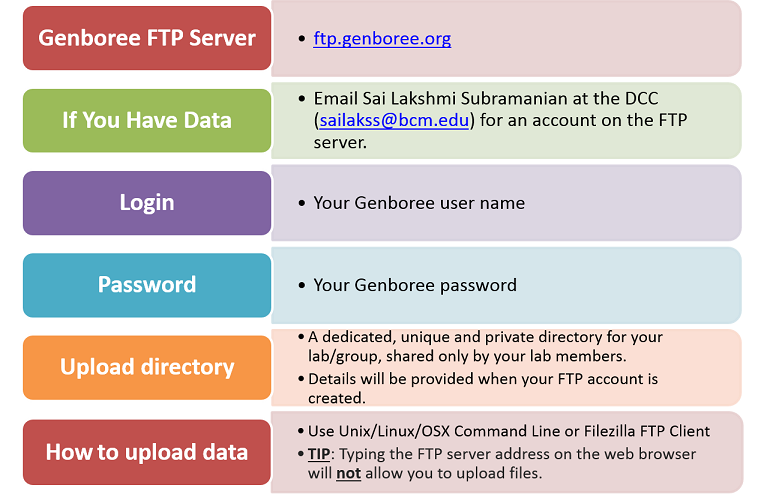
Files Needed for Data Submission
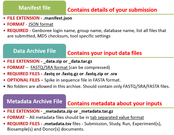


RT-qPCR Data Submission to DCC
Quantitative PCR with reverse transcription is one of the commonly used assay in addition to RNA-sequencing to characterize extracellular RNAs.
This Wiki page includes instructions on how to submit your RT-qPCR data with accompanying metadata to the Data Coordination Center (DCC).
This tutorial will walk you through the entire process of creating an FTP account, formatting and submitting your data and metadata properly,
and then viewing your data in the exRNA Atlas. All submitted samples will be manually curated by the DCC Staff. This is a temporary curation/validation step,
until the FTP Data/Metadata Submission pipeline for qPCR data is made available.
Step 0: Getting an FTP Account on the Genboree FTP Server
Creating Your FTP Account
Files Needed for Data Submission
Your submission will consist of two different files:
- a data archive: - The data archive will contain all of your different data files (RDML format or any other custom format provided by the qPCR instrument).
- a metadata archive: - The metadata archive will contain various metadata documents relating to your data submission.
IMPORTANT NOTE
Both files must have the same basic file name, other than the data archive file name ending in _data and the metadata archive file name ending in _metadata.
This will be explained in more detail below, but your files will look something like this:
- qPCR_samples_data.zip
- qPCR_samples_metadata.zip
Here, I've chosen the name "qPCR_samples" for my submission. This is just an example - you should give a more descriptive name in your actual submission ("alzheimersDiseaseMay2016-UH2_data.zip", for example).
Step 1: Preparing Your Data Archive
Prepare Your qPCR Data Archive
Prepare Your Metadata Archive
You can follow the instructions given in the above link to prepare your metadata documents. Ensure that your metadata contains information relevant to the qPCR assay i.e. all relevant qPCR metadata fields in each collection should be filled out.
This section provides templates for each document type that will allow you to easily and quickly fill out your TSV files using Microsoft Excel or any simple word processor.
 LAST UPDATED: June 22nd, 2016
- If you are interested in building a metadata document, first download the appropriate template ("Biosamples Doc Template" template if you're building a "Biosample" document, for example).
- You can click the link in the column named Template in GenboreeKB UI and use it for preparing your metadata document or checking the correct ontology terms for your metadata property.
- The KB used for these templates is a "testing ground" and will not be used for any final submission of metadata. Feel free to experiment, save your completed template as a document, etc.
- Once you've saved your document, you can download it and use it in your FTP submission (where it will be submitted to the Atlas).
- The Metadata Submission Using GenboreeKB UI page will provide more information on navigating the GenboreeKB UI.
IMPORTANT NOTE: You should be logged in with your Genboree user name and password to use the KB UI.
Step 3: Uploading Your Submission to the FTP Server for Validation
Upload Submission to the DCC
Step 4: Viewing Your Results
Viewing Your qPCR Data in the exRNA Atlas
Miscellaneous Tips and Tricks
Below, you'll find some useful tips and tricks for creating your submission.
Creating an Archive
Creating an Archive
Learning How to Use the Terminal
If you need help navigating the terminal (and want to learn some basic Linux/OSX commands), the following links will be useful:
Overview
Introduction
The exRNA Atlas contains a number of different analysis tools for analyzing Atlas RNA-seq data:
- XDec, a tool for deconvoluting small RNA-seq data from complex biofluids or fractions to estimate the exRNA expression profiles of constituent cargo profiles as well as the per-sample proportions of each constituent cargo profile.
- DESeq2, a differential expression analysis tool
- Dimensionality Reduction Plotting Tool, a visualization tool that allows users to see miRNA expression via PCA and tSNE embedding.
- Generate Summary Report, a tool which summarizes output from multiple samples processed through exceRpt into one cohesive report
Below, we will demonstrate how to use these tools on Atlas data and see your analysis results in the Atlas.
Before we begin describing how to use the analysis tools, we'll go over what each tool does in more detail.
Currently, all analysis tools work solely with RNA-seq profiles.
XDec
- Download an archive containing the results of the deconvolution analysis.
- A full description of the deconvolution method used by XDec can be found in the Cell paper "ExRNA Atlas Analysis Reveals Distinct Extracellular RNA Cargo Types and Their Carriers Present Across Human Biofluids" (Murillo et al., 2019).
- We provide a number of different options for using XDec. The full list of options can be found on the Atlas.
- Tool designed and implemented by Oscar D. Murillo at the Bioinformatics Research Lab, Baylor College of Medicine, Houston, TX.
- Integrated into the exRNA Atlas by William Thistlethwaite at the Bioinformatics Research Lab, Baylor College of Medicine, Houston, TX.
DESeq2
- View a table containing differentially expressed miRNAs for selected Atlas data.
- Sort data by a variety of different metrics (adjusted p-value by default).
- Select some subset of miRNAs and use the Pathway Finder tool to find pathways containing miRNAs of interest (or protein targets of those miRNAs).
- Currently, our integration of the tool allows for pairwise comparisons of sample profiles (two conditions, two RNA isolation kits, etc.).
- Tool designed and implemented by Michael Love, Simon Anders, and Wolfgang Huber (PubMed).
- Integrated into the exRNA Atlas by William Thistlethwaite and Neethu Shah at the Bioinformatics Research Lab, Baylor College of Medicine, Houston, TX.
Dimensionality Reduction Plotting Tool
- Visualize selected Atlas data via PCA and tSNE embedding.
- Choose between three different plotting styles (ggplot2, plotly 2D, and plotly 3D).
- Pick between four different RNA categories (miRNA, piRNA, tRNA, snRNA) for your visualization.
- Color your plots by various metadata categories like dataset, anatomical location, condition, and biofluid name.
- Use filters to add or remove different datasets and biofluids from a given plot (with dynamically adjusted counts for each option).
- Note that these filters are purely visual and do not recompute the PCA or tSNE values.
- Currently, only precomputed analyses are available for this tool.
- Tool designed and implemented by James Diao and Joel Rozowsky at the Gerstein Lab, Yale University, New Haven, CT.
- Integrated into the exRNA Atlas by William Thistlethwaite and Andrew R. Jackson at the Bioinformatics Research Lab, Baylor College of Medicine, Houston, TX.
Generate Summary Report
- Download an archive containing a collection of summary files describing the output from exceRpt for selected samples.
- Summary files include:
- Plots including read count distributions, biotype distributions, miRNA abundance distributions, etc.
- Read count tables for each library (miRNA / tRNA / piRNA / etc.) that span all selected samples. Both raw counts and normalized counts (reads per million mapped reads) are available.
- Visualized taxonomy trees for exogenous rRNA and exogenous genomic reads.
- A full list of summary files can be found on the exceRpt Tutorial Page.
- Tool designed and implemented by Rob Kitchen and Joel Rozowsky at the Gerstein Lab, Yale University, New Haven, CT.
- Integrated into the exRNA Atlas by William Thistlethwaite and Neethu Shah at the Bioinformatics Research Lab, Baylor College of Medicine, Houston, TX.
Viewing Public Analysis Results
Before running your own analyses, you may be interested in viewing the Atlas' public analysis results.
- These results are available to everyone and cover much of the Atlas data.
- They should be useful for an initial examination of what the Atlas has to offer.
To view the Atlas' public analysis results, you can click the Analysis Results button in the Atlas navigation bar and then click the Public Analysis Results button.
You will then be taken to a page where you can click between different tabs, each corresponding to a different tool.
When you click a given tab, you will see the public analysis results associated with that tool:
- The Date column will tell you when the analysis was run.
- The Analysis Name column will tell you the name of the analysis.
- The Samples Processed column will tell you how many samples were involved in the analysis.
- The View Results column will allow you to view the results associated with a given analysis.
- The Load More / Load All buttons will display additional results associated with a given tool (if available).
You can see an example of the public analysis results page below:
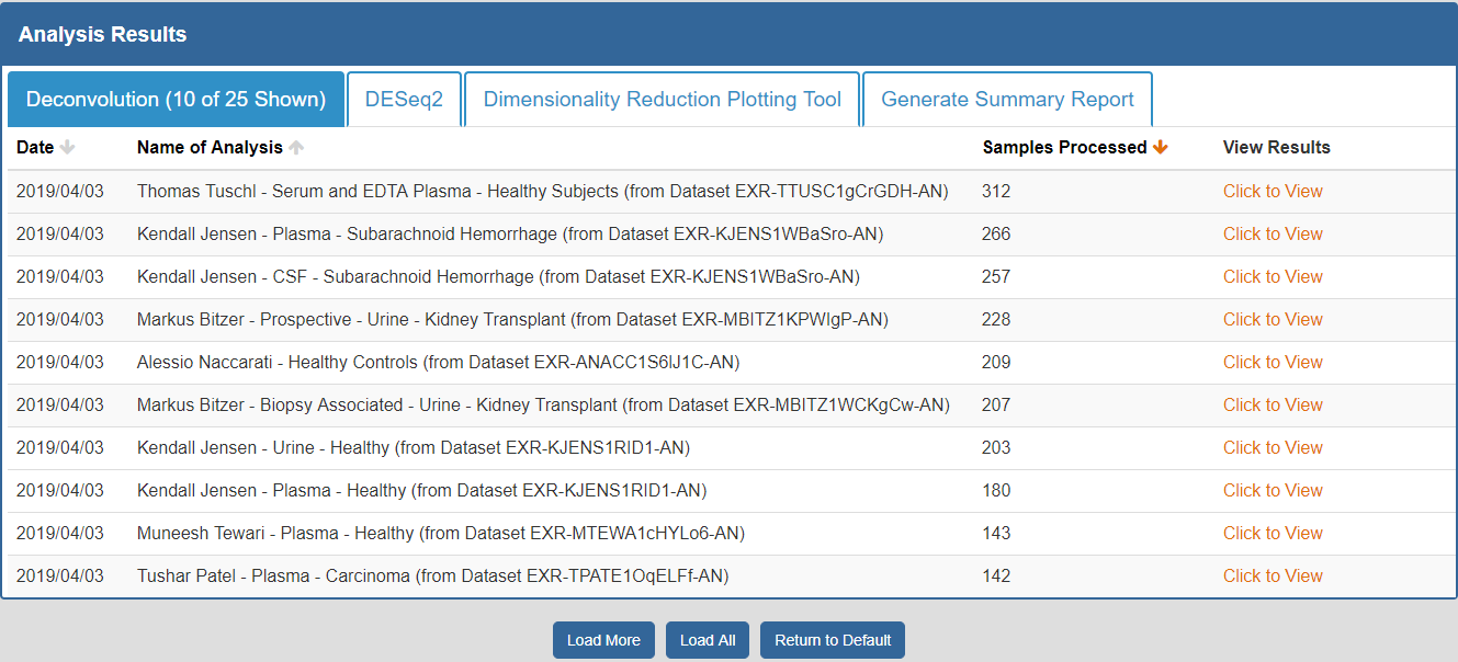
To better understand the output for a given tool, please see the "Understanding Your DESeq2 Results", "Understanding Your Dimensionality Reduction Plotting Tool Results", and "Understanding Your Generate Summary Report Results" sections below.
Running Your Own Analyses
Step 1: Selecting Your Samples of Interest
The first step to running an analysis is selecting your samples of interest.
We recommend using the faceted charts or selecting a dataset from the Datasets page to select your samples (all tools may not be available for other types of grids).
- If using the faceted charts, click the appropriate facets and then click the magnifying glass icon to show corresponding samples in a grid.
- If using the Datasets page, you can click the sample count badge in the lower right corner of a given dataset card to show corresponding samples in a grid.
Below, you can see an example of how one would select samples via the faceted charts:
And here is an example of how one would select a set of samples via the Datasets page:
After you have generated your grid, you will need to select the specific samples you want to analyze.
- You can select specific samples by using the checkboxes to the left of each sample.
- To select all samples, click the checkbox in the upper left corner of the grid.
- The different metadata columns (Condition, Anatomical Location, etc.) should help you figure out which specific samples you want to analyze.
- You can also click on the right side of a given column to sort that column, place filters on that column, or disable any column in the grid.
Below, you can see an example where I've selected 4 samples in my samples grid:
After you've selected your samples, you'll need to pick out a tool to run on those samples.
You can click the "Analyze Selected Samples" button to see available tools.
- You can read more about the individual tools in the Overview of Tools section above.
After choosing a tool, you will be prompted to log into your Genboree account (unless you are already logged in).
- A Genboree account is required to use the analysis tools.
- If you have an account already, just fill in your login information and then click the "Login" button.
- If you don't have an account, you can click the "Register here!" link to create one.
- Once you've logged in once, you won't need to log in again for that Atlas session.
After you've logged in, you'll be prompted to provide settings for your analysis run.
- First, you'll need to select a Group and Database in which to store your output files.
Each Genboree account starts with a Group (named after your username), and we will offer to create a Database for you (named "Exrna-atlas Output") if you don't have one.
- Next, you'll need to provide an Analysis Name for your analysis run - this name will be used to organize your analysis results, so picking an informative name is a good idea!
- Finally, some tools will require additional settings - for example, DESeq2 will require you to put in a factor name and two factor levels of interest.
When you're ready to submit your analysis, click the Submit Analysis button.
After a moment, you will be provided an analysis job ID. You will receive an email when your analysis run is complete.
Step 3: Viewing Your Analysis Results
To view your analysis results, you can click the Analysis Results button in the Atlas navigation bar and then click the My Analysis Results button.
You will then be taken to a page where you can click between different tabs, each corresponding to a different tool.
When you click a given tab, you will see any analysis results associated with that tool:
- The Date column will tell you when the analysis was run.
- The Analysis Name column will tell you the name of the analysis.
- The Samples Processed column will tell you how many samples were involved in the analysis.
- The View Results column will allow you to view the results associated with a given analysis.
- The Load More / Load All buttons (if available) will display additional results associated with a given tool.
You can see an example of an analysis results page below:
To better understand the output for a given tool, please see the "Understanding Your DESeq2 Results" and "Understanding Your Generate Summary Report Results" sections below.
Understanding Your Results
Understanding Your XDec Results
Output from XDec includes:
- Stage 1 Deconvolution
- Heatmap representing the correlation between the deconvoluted cargo profiles modeled for the current dataset and the cargo types (CT) estimated from the deconvolution of individual Atlas datasets across informative ncRNAs.
- Table of estimated constituent cargo profiles across 20,000+ ncRNA [miRNA, piRNA, tRNA, Y RNA, lincRNA, snoRNA, snRNA] transcripts (expression is normalized to [0:1] range).
- Heatmap representing the proportions of each cargo profile for each sample in the current dataset.
- Table of estimated proportions of each cargo profile for each sample in the current dataset.
- Boxplots representing the proportions of each cargo profile for each sample in the current dataset separated based on provided metadata features.
- Stage 2 Deconvolution
- Tables of estimated average cargo profiles across 20,000+ ncRNA (miRNA, piRNA, tRNA, Y RNA, lincRNA, snoRNA, and snRNA) transcripts in reads per million (RPM) separated based on provided metadata features. Tables include mean expression, std. errors, degrees of freedom, and per sample residuals.
To learn more about XDec and how to interpret your results, read the Cell paper "ExRNA Atlas Analysis Reveals Distinct Extracellular RNA Cargo Types and Their Carriers Present Across Human Biofluids" (Murillo et al., 2019).
Understanding Your DESeq2 Results
When you click to view your DESeq2 results, a new page will open up containing differentially expressed miRNAs for the selected Atlas data.
Each row corresponds to a given miRNA, and each column is explained below:
- The Checkbox column allows you to select miRNAs for further downstream analysis.
- You can click the checkbox next to a given miRNA (highlighted in blue below) to select that miRNA.
- You can click the checkbox in the upper left corner of the table (highlighted in green below) to select all visible miRNAs.
- The Identifiers column contains all of your miRNA identifiers.
- The Base Mean column contains "the average of the normalized count values, divided by the size factors, taken over all samples [in the original dataset]" for each miRNA. [1]
- The log2 Fold Change column contains the "effect size estimate" for each miRNA. [1]
- The Standard Error column contains the "standard error estimate for the log2 fold change estimate" for each miRNA. [1]
- The p-value column contains the Wald test p-value for each miRNA. [1]
- The Adjusted p-value column contains the Benjamini-Hochberg adjusted p-value for each miRNA. [1]
[1] Love, M. I., Anders, S., Kim V., & Huber W. (2017, Aug 9). RNA-seq workflow: gene-level exploratory analysis and differential expression.
Retrieved from http://www.bioconductor.org/help/workflows/rnaseqGene/
By default, the table is sorted by adjusted p-value, but you can sort by any of the columns.
In addition, you can perform downstream analysis on selected miRNAs of interest by clicking the Analyze Selected miRNAs button (highlighted in red below) above the table.
See descriptions of all available downstream analysis tools below.
Pathway Finder
- Use Pathway Finder (hosted by WikiPathways) to find pathways containing miRNAs of interest (or protein targets of those miRNAs).
- Click a given pathway title to visualize its contents at the bottom of the page.
- Then, select a given miRNA to highlight its associated target(s).
- The pathway visualization is interactive - zoom in or out by using the + and - icons, and click a given gene product to learn more about it.
- Designed and implemented by Kristina Hanspers, Anders Riutta, and Alexander Pico at the Gladstone Institutes, San Francisco, CA.
- Integrated into the exRNA Atlas by William Thistlethwaite and Neethu Shah at the Bioinformatics Research Lab, Baylor College of Medicine, Houston, TX.
You can see what the Pathway Finder interface looks like below:
When you click to view your Dimensionality Reduction Plotting Tool results, a new page will open up containing an interface for visualizing the expression of different ncRNAs in the selected Atlas data.
On the left side of the screen, you will see the Control Panel and Filtering Panel that allow you to configure your visualization.
Within the Control Panel, you will see the following settings:
- The Plotting Style setting allows you to choose between two different plotting tools (ggplot2 and plotly).
- Note that ggplot2 supports 2D plots while plotly supports both 2D and 3D plots.
- The Embedding setting allows you to choose between PCA and tSNE embedding.
- If you currently have PCA selected, you can choose between the top 5 principal components using the Principal Components setting.
- The RNA Category setting allows you to choose the type of ncRNA you'd like to plot.
- The Color By setting allows you to choose how you'd like to color your plot.
Within the Filtering Panel, you will see the following settings:
- The Datasets setting allows you to to add or remove different datasets from your plot (with dynamically adjusted counts for each option).
- Note that these filters are purely visual and do not recompute the PCA or tSNE values.
- The Biofluids setting allows you to to add or remove different biofluids from your plot (with dynamically adjusted counts for each option).
- Note that these filters are purely visual and do not recompute the PCA or tSNE values.
After you've selected your settings, you can click the Make New Plot button on the right side of the screen to generate a new visualization based on your current Control Panel and Filtering Panel settings.
You can then download a PDF of your current visualization by clicking the Download Plot button.
Understanding Your Generate Summary Report Results
When you click to view your Generate Summary Report results, you will download an archive containing a variety of summary files describing the selected Atlas data.
Descriptions of the summary files can be found below:
| File Name |
Description of File |
| QC Data |
|
| [analysisName]_exceRpt_DiagnosticPlots.pdf |
All diagnostic plots automatically generated by the tool |
| [analysisName]_exceRpt_readMappingSummary.txt |
Read-alignment summary including total counts for each library |
| [analysisName]_exceRpt_ReadLengths.txt |
Read-lengths (after 3' adapters/barcodes are removed) |
| [analysisName]_exceRpt_QCresults.txt |
QC statistics for all samples |
| Raw Transcriptome Quantifications |
|
| [analysisName]_exceRpt_miRNA_ReadCounts.txt |
miRNA read-counts quantifications |
| [analysisName]_exceRpt_tRNA_ReadCounts.txt |
tRNA read-counts quantifications |
| [analysisName]_exceRpt_piRNA_ReadCounts.txt |
piRNA read-counts quantifications |
| [analysisName]_exceRpt_gencode_ReadCounts.txt |
gencode read-counts quantifications |
| [analysisName]_exceRpt_circularRNA_ReadCounts.txt |
circularRNA read-count quantifications |
| [analysisName]_exceRpt_biotypeCounts.txt |
biotype read-count quantifications |
| [analysisName]_exceRpt_exogenous_miRNA_ReadCounts.txt |
exogenous miRNA read-counts quantifications |
| Normalized Transcriptome Quantifications |
|
| [analysisName]_exceRpt_miRNA_ReadsPerMillion.txt |
miRNA RPM quantifications |
| [analysisName]_exceRpt_tRNA_ReadsPerMillion.txt |
tRNA RPM quantifications |
| [analysisName]_exceRpt_piRNA_ReadsPerMillion.txt |
piRNA RPM quantifications |
| [analysisName]_exceRpt_gencode_ReadsPerMillion.txt |
gencode RPM quantifications |
| [analysisName]_exceRpt_circularRNA_ReadsPerMillion.txt |
circularRNA RPM quantifications |
| [analysisName]_exceRpt_exogenous_miRNA_ReadsPerMillion.txt |
exogenous miRNA RPM quantifications |
| Exogenous Genomic Taxonomies |
|
| [analysisName]_exceRpt_exogenousGenomes_taxonomyCumulative_ReadCounts.txt |
cumulative taxonomy read-count quantifications |
| [analysisName]_exceRpt_exogenousGenomes_taxonomyCumulative_ReadsPerMillion.txt |
cumulative taxonomy RPM quantifications |
| [analysisName]_exceRpt_exogenousGenomes_taxonomySpecific_ReadCounts.txt |
specific taxonomy read-count quantifications |
| [analysisName]_exceRpt_exogenousGenomes_taxonomySpecific_ReadsPerMillion.txt |
specific taxonomy RPM quantifications |
| [analysisName]_exceRpt_exogenousGenomes_TaxonomyTrees_aggregateSamples.pdf |
visualized taxonomy tree for samples, aggregated |
| [analysisName]_exceRpt_exogenousGenomes_TaxonomyTrees_perSample.pdf |
visualized taxonomy trees for each sample |
| Exogenous rRNA Taxonomies |
|
| [analysisName]_exceRpt_exogenousRibosomal_taxonomyCumulative_ReadCounts.txt |
cumulative taxonomy read-count quantifications |
| [analysisName]_exceRpt_exogenousRibosomal_taxonomyCumulative_ReadsPerMillion.txt |
cumulative taxonomy RPM quantifications |
| [analysisName]_exceRpt_exogenousRibosomal_taxonomySpecific_ReadCounts.txt |
specific taxonomy read-count quantifications |
| [analysisName]_exceRpt_exogenousRibosomal_taxonomySpecific_ReadsPerMillion.txt |
specific taxonomy RPM quantifications |
| [analysisName]_exceRpt_exogenousRibosomal_TaxonomyTrees_aggregateSamples.pdf |
visualized taxonomy tree for samples, aggregated |
| [analysisName]_exceRpt_exogenousRibosomal_TaxonomyTrees_perSample.pdf |
visualized taxonomy trees for each sample |
| R Objects |
|
| [analysisName]_exceRpt_smallRNAQuants_ReadCounts.RData |
All raw data (binary R object) |
| [analysisName]_exceRpt_smallRNAQuants_ReadsPerMillion.RData |
All normalized data (binary R object) |
| Other |
|
| [analysisName]_exceRpt_sampleGroupDefinitions.txt |
Information about sample groups (not used by Atlas) |
Below, you can see some example plots from the Diagnostic Plots PDF referenced above.
Microsoft Excel in Windows
Select "Save As" from the menubar.
Navigate to the folder where you would like to save your metadata document.
Provide a file name for your document. Remember, file names end with .metadata.tsv.
Select the option "Text (Tab delimited)" from the pull down menu for "Save as type" and press OK.
Microsoft Excel in Mac
To save your metadata documents as a properly formatted tab-separated value file, click "Save" and
select the option to save as "Windows Formatted Text".
This option saves the file as a tab-separated value file without any special characters.
LibreOffice Calc
Select "Save As", choose "All Format", and then choose "Test CSV (.csv)".
You will see a dialog box titled "Export Text File".
Select {Tab} from the pull down menu for "Field delimiter" and select OK.
Your document will be saved as a tab-delimited text file.
Sanity Check the TSV file
To ensure there are no special characters in your metadata document after following the above mentioned
methods to save your file, open the document in any text editor like
- Notepad (Windows),
- gedit (Ubuntu/Linux),
- TextEdit (Mac) or
- command line editors like vim, nano, etc. in the Terminal (Linux/Unix/Mac OSX).
Check if the document is properly formatted, i.e. columns are separated by a tab character and
the document does not have any characters like ^M, etc.
Troubleshooting
- Your submission may fail even after you take a considerable amount of time formatting your files. Don't fret!
- There are a couple of steps you can take if you receive a failure e-mail:
- Read the error message at the bottom of the e-mail and see if it is informative.
- Often times, if there is an error in one or more of your metadata files, the error e-mail will tell you exactly why the pipeline failed.
- If the error message isn't helpful or you're still perplexed, feel free to send an e-mail to Emily to get some help.
- We check each part of your submission (manifest file / metadata archive / data archive) in order.
If any of your submitted files are unchecked or pass inspection, they will be moved back to your lab's submission inbox.
- For example, if there are errors in your manifest file, we will automatically move your metadata archive and data archive back to your submission inbox.
- This makes the submission process easier, since you don't have to keep uploading your files or moving them around on the FTP server.
- In each metadata file, you will have a "#property" column and at least one "value" column.
- The "#property" column contains different metadata properties, and the "value" column contains values for those metadata properties.
- For each entry in the "#property" column, you'll notice that different properties have different numbers of dashes and stars preceding the actual property names.
- These "-" and "*" symbols serve as nesting prefixes.
- When a given property is nested underneath another property, that means the first property is a subproperty of the second property.
- The subproperty usually provides more detail about the parent property in some way.
- You can see an example to better understand the nested tabbed format.
The Symbol -
- The symbol "-" indicates an additional basic level of nesting for a given property. For example, see the table below:
| #property |
value |
| -- Biological Fluid |
|
| --- Biofluid Name |
serum |
| --- Collection Details |
|
| ---- Sample Collection Method |
venipuncture |
- Here, --- Biofluid Name and --- Collection Details are nested under -- Biological Fluid, and ---- Sample Collection Method is nested under --- Collection Details.
- The Biofluid Name and Collection Details properties provide more information about the Biological Fluid property, and the Sample Collection Method property provides more information about the Collection Details property.
The Symbol *
- The symbol "*" indicates that the property contains an item list.
- This list can be as long as you like, and each property name will be the same within the list.
- For example: Imagine that you have 4 authors associated with your study. There is a property named * Authors in your Studies metadata file.
Below this property, there will be 1 row for the *- Author Name property. This property is an item in the * Authors item list.
If you want to add 3 more authors, simply add another 3 rows of *- Author Name, like so:
| #property |
value |
| * Authors |
|
| *- Author Name |
NAME1 |
| *- Author Name |
NAME2 |
| *- Author Name |
NAME3 |
| *- Author Name |
NAME4 |
Upload longRNAseq Submission to the DCC using FTP Server
Below, we give two different ways of uploading your files:
- LFTP command line client (Linux / Unix / Mac)
- FileZilla
Please contact us at brl-exrna@bcm.edu if your data archive is over 100GBs.
Uploading Submission via the LFTP Command Line Client (Linux / Unix / Mac)
Step 1. Setup
- Open up a terminal and navigate to the directory on your local computer that contains the 3 files that you're going to submit.
- Type "lftp ftps://ftps.genboree.org -u [username]" to connect to our FTPs server, where [username] is your FTP login or Genboree username.
- When prompted, enter your FTP password (Genboree password).
- Navigate to your lab's private directory. You can do this by typing "cd [PRIVATE_DIR]", where [PRIVATE_DIR] is your lab's private directory (given to you via e-mail).
- Next, navigate to your lab's inbox directory by typing "cd inbox/".
Step 2. Uploading Your Files
- Use the "put" command to upload your files by typing "put" followed by the respective names of your manifest file, metadata archive, and data archive.
- Type "ls" to ensure all your files have been copied and the file size of the copied file is same as the original file size.
- After the file transfers are complete, type "exit" to exit the lftp client.
Example
Imagine that I had the following set of three files:
- Manifest named
test_longRNAseq.manifest.json
- Metadata archive named
test_longRNAseq_metadata.zip
- Data archive named
test_longRNAseq_data.zip
Furthermore, all 3 files are stored at the following location on my local computer: /home/myHome/myDataDir/smallRNASeqData.
I would perform the following commands to upload all three files to the FTP server (replacing PICODE with whatever my PI code is):
cd /home/myHome/myDataDir/longRNASeqData
lftp ftps://ftps.genboree.org -u username
# enter password
cd exrna-PICODE/
cd inbox/
put test_longRNAseq.manifest.json test_longRNAseq_metadata.zip test_longRNAseq_data.zip
ls
exit
Please note that any lines that begin with # are comments and are not actual commands that you should type!
For example, you shouldn't actually type "# enter login name and password" - that's just me informing you that
you'll need to enter your password after the "lftp ftps://ftps.genboree.org -u <user name>" command.
Uploading Submission via the FileZilla FTP Client
Step 1. Setup
- Download and install the FileZilla Client.
- After opening the client, make sure that you change your transfer type to binary mode (from the default type of Auto).
This is done to ensure that your files are uploaded properly to our server.
To change your transfer type, go to the menu bar at the top of the window and select the following:
Transfer -> Transfer type -> Binary.
- Fill in the following information just below the menu bar:
- Click "Quickconnect" to connect to the FTP server.
- You will see your own files displayed on the left side of the window ("Local site") and the FTP server's files displayed on the right side of the window ("Remote site").
Step 2. Uploading Your Files
- Navigate to the directory that contains your metadata archive and data archive using the left side of the window.
- Navigate to your upload directory (unique and private to your lab/group) using the right side of the window.
- Drag and drop your submission (which should consist of two files) from the lower left panel to the lower right panel.
- Once your transfer is successful (you can see the progress of your transfer in the panel at the bottom of the window), close FileZilla - you're done!
Resuming File Upload (If Upload Fails)
If your transfer fails before it completes, you will need to resume it from the point where it failed.
- When you open FileZilla, there should be information about incompletely transferred files in the bottom panel of the window (under "Queued files").
- Right click anywhere in that panel and click "Process Queue". Make sure that you type your password in when requested.
- Select the action "Resume" from the options listed and click OK.
- Repeat this last step for each file that you want to resume.
(If the file transfer completes after resuming from a previous transfer and the MD5 does not match to what you have provided, please remove the file and start from step 2 again.)
Send an email to notify us
- Once all three files have been uploaded, please send an email at brl-exrna@bcm.edu with your private lab folder name and file names.
Sending the data via a hard drive
Please coordinate with us at brl-exrna@bcm.edu and provide the following information prior to sending the hard drive
- PI name
- Name of the study
- total number of samples
- size of the data archive (GBs/TBs?)
Copy the data archive, metadata, and manifest into the external hard drive
- make sure the data archive is transferred correctly by checking the MD5 checksum of the file on the external hard drive.
- Send the hard drive to:
David Chen
C/O BRL@ Baylor College of Medicine
1 Baylor Plaza
Jewish Building 400DM
Houston, TX 77030
Notify us that you are sending the hard drive by emailing us at brl-exrna@bcm.edu with the tracking number and the return information.
Upload qPCR Submission to the DCC using FTP Server
Below, we give two different ways of uploading your files:
- FileZilla (recommended and very easy to use!)
- FTP command line client (Linux / Unix / Mac)
- Note that the Windows command line client is not supported.
Uploading Submission via the FileZilla FTP Client
Step 1. Setup
- Download and install the FileZilla Client.
- After opening the client, make sure that you change your transfer type to binary mode (from the default type of Auto).
This is done to ensure that your files are uploaded properly to our server.
To change your transfer type, go to the menu bar at the top of the window and select the following:
Transfer -> Transfer type -> Binary.
- Fill in the following information just below the menu bar:
- Click "Quickconnect" to connect to the FTP server.
- You will see your own files displayed on the left side of the window ("Local site") and the FTP server's files displayed on the right side of the window ("Remote site").
Step 2. Uploading Your Files
- Navigate to the directory that contains your metadata archive and data archive using the left side of the window.
- Navigate to your upload directory (unique and private to your lab/group) using the right side of the window.
- Drag and drop your submission (which should consist of two files) from the lower left panel to the lower right panel.
- Once your transfer is successful (you can see the progress of your transfer in the panel at the bottom of the window), close FileZilla - you're done!
Resuming File Upload (If Upload Fails)
If your transfer fails before it completes, you can easily resume it from the point where it failed.
- When you open FileZilla, there should be information about incompletely transferred files in the bottom panel of the window (under "Queued files").
- Right click anywhere in that panel and click "Process Queue". Make sure that you type your password in when requested.
- Select the action "Resume" from the options listed and click OK.
- Repeat this last step for each file that you want to resume.
Uploading Submission via the FTP Command Line Client (Linux / Unix / Mac)
Step 1. Setup
- Open up a terminal and navigate to the directory on your local computer that contains the 3 files that you're going to submit.
- Type "ftp ftp.genboree.org" to connect to our FTP server.
- When prompted, enter your FTP login (Genboree username) and FTP password (Genboree password).
- Switch to binary transfer mode by typing "bin" - this will ensure that your files are transferred correctly.
- Navigate to your lab's private directory. You can do this by typing "cd [PRIVATE_DIR]", where [PRIVATE_DIR] is your lab's private directory (given to you via e-mail).
- Next, navigate to your lab's inbox directory by typing "cd inbox/".
- Type "prompt" to switch off confirmation for each file uploaded.
Step 2. Uploading Your Files
- Use the "mput" command to upload your files by typing "mput" followed by the respective names of your metadata archive and data archive.
- Type "dir" to ensure all your files have been copied and the file size of each copied file is same as the original file size.
- After the file transfers are complete, type "bye" to exit the FTP client.
Example
Imagine that I had the following set of three files:
- Manifest file named
test_qPCR.manifest.json
- Metadata archive named
test_qPCR_metadata.zip
- Data archive named
test_qPCR_data.zip
Furthermore, all three files are stored at the following location on my local computer: /home/myHome/myDataDir/qPCRData.
I would perform the following commands to upload all three files to the FTP server (replacing PICODE with whatever my PI code is):
cd /home/myHome/myDataDir/qPCRData
ftp ftp.genboree.org
# enter login name and password
bin
cd exrna-PICODE/
cd inbox/
prompt
mput test_qPCR.manifest.json test_qPCR_metadata.zip test_qPCR_data.zip
dir
bye
Please note that any lines that begin with # are comments and are not actual commands that you should type!
For example, you shouldn't actually type "# enter login name and password" - that's just me informing you that
you'll need to enter your login name and password after the "ftp ftp.genboree.org" command.
Resuming File Uploads (If Upload Fails)
If your upload fails and you want to resume it, you will need to reconnect to the FTP server and navigate back to your
upload directory (remember to type "bin" and "prompt" just like before!).
- Check the file size of your partially-transferred files by typing "dir". You can compare their respective
byte sizes with your local versions of the files - if the versions on the FTP server are smaller, that means that the files were
only partially transferred. For each partially transferred file, you will want to complete the following process:
- Type "restart" followed by the total number of bytes in the partially-transferred file.
- Example: If my partially-transferred file was 1000 bytes, I would type "restart 1000".
- Type "put", hit enter, and then fill in the name of the file, when prompted, for both local and remote. You will put the
same name ("test_qPCR_data.zip", for example) for both local and remote.
- Type "dir" to check that the file transfer completed successfully, and then type "bye" to log off.
ftp ftp.genboree.org
# enter login name and password
bin
cd exrna-PICODE/
cd inbox/
prompt
dir
# to restart uploading a partially transferred file with file size 1000 bytes
restart 1000
put
FILENAME
FILENAME
dir
bye
Send an email to notify us
- Once all three files have been uploaded, please send an email at brl-exrna@bcm.edu with your private lab folder name and file names.
Below, we give two different ways of uploading your files:
- LFTP command line client (Linux / Unix / Mac)
- FileZilla
Please contact us at brl-exrna@bcm.edu if your data archive is over 100GBs.
Uploading Submission via the LFTP Command Line Client (Linux / Unix / Mac)
Step 1. Setup
- Open up a terminal and navigate to the directory on your local computer that contains the 3 files that you're going to submit.
- Type "lftp ftps://ftps.genboree.org -u [username]" to connect to our FTPs server, where [username] is your FTP login or Genboree username.
- When prompted, enter your FTP password (Genboree password).
- Navigate to your lab's private directory. You can do this by typing "cd [PRIVATE_DIR]", where [PRIVATE_DIR] is your lab's private directory (given to you via e-mail).
- Next, navigate to your lab's inbox directory by typing "cd inbox/".
- Type "prompt" to switch off confirmation for each file uploaded.
Step 2. Uploading Your Files
- Use the "put" command to upload your files by typing "put" followed by the respective names of your manifest file, metadata archive, and data archive.
- Type "ls" to ensure all your files have been copied and the file size of the copied file is same as the original file size.
- After the file transfers are complete, type "exit" to exit the FTP client.
Example
Imagine that I had the following set of three files:
- Manifest named
test.manifest.json
- Metadata archive named
test_metadata.zip
- Data archive named
test_data.zip
Furthermore, all 3 files are stored at the following location on my local computer: /home/myHome/myDataDir/smallRNASeqData.
I would perform the following commands to upload all three files to the FTP server (replacing PICODE with whatever my PI code is):
cd /home/myHome/myDataDir/smallRNASeqData
lftp ftps://ftps.genboree.org -u username
# enter password
cd exrna-PICODE/
cd inbox/
put test.manifest.json test_metadata.zip test_data.zip
ls
exit
Please note that any lines that begin with # are comments and are not actual commands that you should type!
For example, you shouldn't actually type "# enter login name and password" - that's just me informing you that
you'll need to enter your password after the "lftp ftps://ftps.genboree.org -u <user name>" command.
Uploading Submission via the FileZilla FTP Client
Step 1. Setup
- Download and install the FileZilla Client.
- After opening the client, make sure that you change your transfer type to binary mode (from the default type of Auto).
This is done to ensure that your files are uploaded properly to our server.
To change your transfer type, go to the menu bar at the top of the window and select the following:
Transfer -> Transfer type -> Binary.
- Fill in the following information just below the menu bar:
- Click "Quickconnect" to connect to the FTP server.
- You will see your own files displayed on the left side of the window ("Local site") and the FTP server's files displayed on the right side of the window ("Remote site").
Step 2. Uploading Your Files
- Navigate to the directory that contains your manifest file, metadata archive, and data archive using the left side of the window.
- Navigate to your upload directory (unique and private to your lab/group) using the right side of the window.
- This directory will look something like "/exrna-amilo1/inbox"
- Drag and drop your submission (which should consist of three files) from the lower left panel to the lower right panel.
- Once your transfer is successful (you can see the progress of your transfer in the panel at the bottom of the window), close FileZilla - you're done!
Resuming File Upload (If Upload Fails)
If your transfer fails before it completes, you can easily resume it from the point where it failed.
- When you open FileZilla, there should be information about incompletely transferred files in the bottom panel of the window (under "Queued files").
- Right click anywhere in that panel and click "Process Queue". Make sure that you type your password in when requested.
- Select the action "Resume" from the options listed and click OK.
- Repeat this last step for each file that you want to resume.
(If the file transfer completes after resuming from a previous transfer and the MD5 does not match to what you have provided, please remove the file and start from step 2 again.)
Send an email to notify us
- Once all three files have been uploaded, please send an email at brl-exrna@bcm.edu with your private lab folder name and file names.
Sending the data via a hard drive
Please coordinate with us at brl-exrna@bcm.edu and provide the following information prior to sending the hard drive
- PI name
- Name of the study
- total number of samples
- size of the data archive (GBs/TBs?)
Copy the data archive, metadata, and manifest into the external hard drive
- make sure the data archive is transferred correctly by checking the MD5 checksum of the file on the external hard drive.
- Send the hard drive to:
David Chen
C/O BRL@ Baylor College of Medicine
1 Baylor Plaza
Jewish Building 400DM
Houston, TX 77030
Notify us that you are sending the hard drive by emailing us at brl-exrna@bcm.edu with the tracking number and the return information.
Introduction to the ncRNA Search Bar
The ncRNA search bar is designed to drill down on an ncRNA-specific level into the Atlas data.
For example, imagine I was very interested in the mature miRNAs hsa-miR-320a and hsa-miR-100-5p.
It would be nice if I could learn more about those mature miRNAs in the context of the Atlas.
Below, we'll learn exactly how to do that.
You can find the ncRNA search bar near the top of the Atlas home page. There are many ways to reach it:
- Click the banner at the top of any page on the Atlas
- Click the Home button in the navigation bar at the top of any page on the Atlas
- Click Select Profiles in the navigation bar and then click ncRNA Search Bar
Below, you can see a picture of the ncRNA search bar (boxed in red):
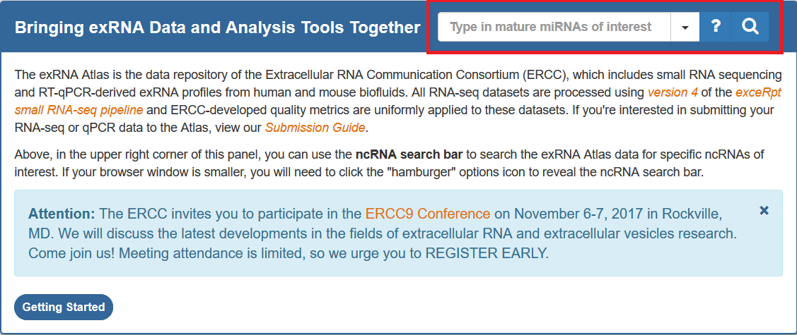
Currently, the ncRNA search bar supports mature miRNAs, tRNAs, and piRNAs.
We recommend the following steps when learning how to use the search bar:
- Click the options icon directly to the right of the text box.
- You can select the type of ncRNA that you'd like to search for (mature miRNA, tRNA, piRNA).
- You can also select your desired database, but we currently only offer one (the Atlas Census, which will be explained further below).
- Once you've selected your type of ncRNA, you can type or paste your identifiers of interest into the text box.
- If you're not sure about how to format your identifiers, you can click the question mark button to bring up a help dialog.
- This help dialog will include example queries for each type of ncRNA, and you can even run an example query by clicking the "Run Example Query" button.
- Once you've written your identifiers of interest, you can click the magnifying glass (or hit enter) to perform your search.
- If you wrote any incorrectly formatted identifiers, an error page will be displayed with some helpful information.
- This error page will include the source database for the type of ncRNA, an example query, and other miscellaneous information.
- You will also see a list of correctly formatted identifiers and a list of incorrectly formatted identifiers.
- If you want, you can click the orange search text in the error panel to directly search for your correctly formatted identifiers (discarding the incorrect ones).
Below, we can see that I've typed three mature miRNA IDs into the search bar:
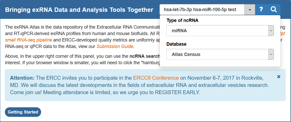
Two of these mature miRNA IDs are valid (hsa-let-7b-3p and hsa-miR-101-5p), while one is invalid (test).
When we click search, we'll see a page like this:

You can see that the page presents some useful information that will help us format our search correctly.
You can use this information to fix your incorrect identifiers, or, if preferred, just directly submit a search with your correct identifiers.
Once you've submitted a properly formatted request, a results page will be displayed.
We will break down the results pages for the different databases below.
Atlas Census
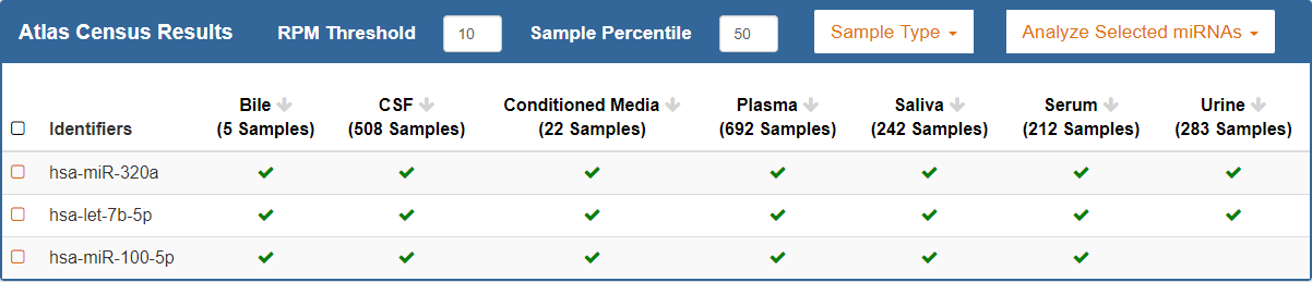
Introduction
When you perform a search using the Atlas Census database, your results will consist of a table that summarize the frequency of your selected ncRNAs in the exRNA Atlas data.
- Each row in the table will correspond to a selected ncRNA.
- Each column in the table will correspond to a biofluid found in the Atlas.
- The number of samples present for each biofluid will be displayed below the name of the biofluid.
- A checkmark in a given cell will indicate that the ncRNA was expressed in that biofluid according to the provided parameters.
- The absence of a checkmark does not mean that the ncRNA was not expressed in that biofluid.
- You can click a biofluid's column header to sort your results by that biofluid.
The parameters listed below will normally be displayed above the table. However, if your browser window isn't large enough to fit the parameters,
a hamburger menu will be made available in the upper right corner. Simply click the hamburger icon to reveal the different parameters.
Parameters for Adjusting Stringency for Detection
There are two parameters for adjusting stringency for detection of your ncRNAs:
- RPM Threshold: For a given ncRNA in a given sample, what RPM (reads per million mapped reads) is required in order for that ncRNA to be considered expressed?
- Sample Percentile: For a given ncRNA in a given biofluid, the sample percentile controls the percentage of samples that must meet the RPM threshold in order for that ncRNA to be considered expressed in that biofluid.
Parameters for Adjusting Sample Subsets
You can also pick different subsets of the Atlas data for your table by using the Sample Type option.
- For example, if you choose Healthy Samples, only healthy samples will be used when generating the table. More options will be coming soon.
- The number of samples below each biofluid will be updated accordingly after picking your new sample type.
Downstream Analysis (for Mature miRNAs)
Finally, if you searched for mature miRNAs (as opposed to tRNAs or piRNAs), you can perform downstream analysis on those mature miRNAs.
First, select your miRNAs of interest (via the checkboxes on the left side of the table).
You can then click the Analyze Selected miRNAs button above the table to see the different downstream analysis tools.
- Pathway Finder
- Use Pathway Finder (hosted by WikiPathways) to find pathways containing miRNAs of interest (or protein targets of those miRNAs).
- Click a given pathway title to visualize its contents at the bottom of the page.
- Then, select a given miRNA to highlight its associated target(s).
- The pathway visualization is interactive - zoom in or out by using the + and - icons, and click a given gene product to learn more about it.
- Designed and implemented by Kristina Hanspers, Anders Riutta, and Alexander Pico at the Gladstone Institutes, San Francisco, CA.
- Integrated into the exRNA Atlas by William Thistlethwaite and Neethu Shah at the Bioinformatics Research Lab, Baylor College of Medicine, Houston, TX.
Viewing All Biosamples in Biosample Partition Grid
As an alternative to the facet search, you can also view all biosamples in one of our biosample partition grids.
We have two different biosample partition grids available: Biofluid vs Condition and Biofluid vs Assay Type.
You can access these grids in two different ways:
First, you can click Select Profiles in the navigation bar and then click Biofluid vs Condition Grid or Biofluid vs Assay Type Grid.
Second, you can use the links on the front page in the Browse exRNA Profiles - Alternative Options panel:
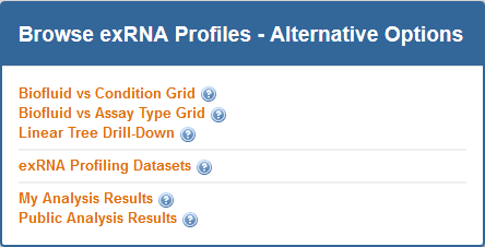
For example, see the Biofluid vs. Condition grid below:
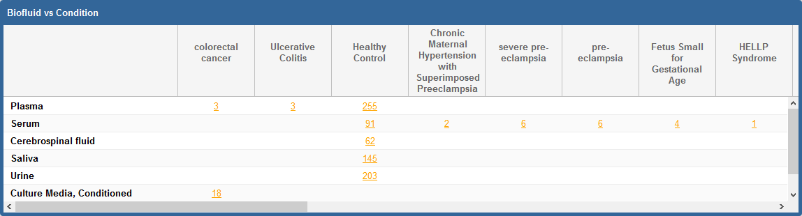
Each cell in this grid indicates the total number of biosamples collected and profiled for exRNAs from a biofluid-condition combination.
If you click the number in a given cell, you will be able to see key metadata about all the biosamples that meet the biofluid-condition criteria given for that cell.
The Biofluid vs. Assay Type grid is very similar except its columns are assay types instead of conditions.
Once you click the number in a given cell, a new grid will be displayed that contains information about associated samples.
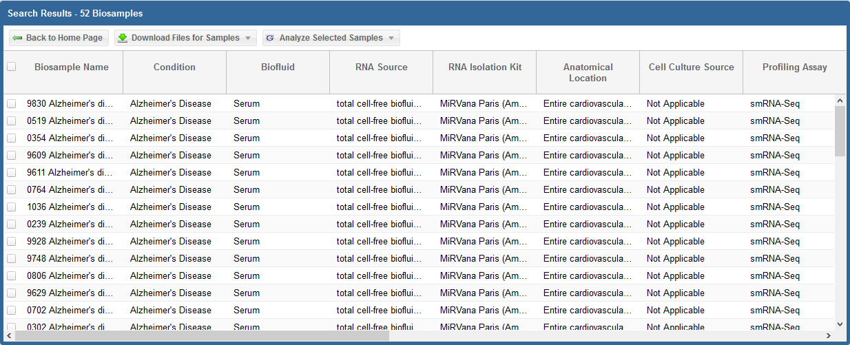
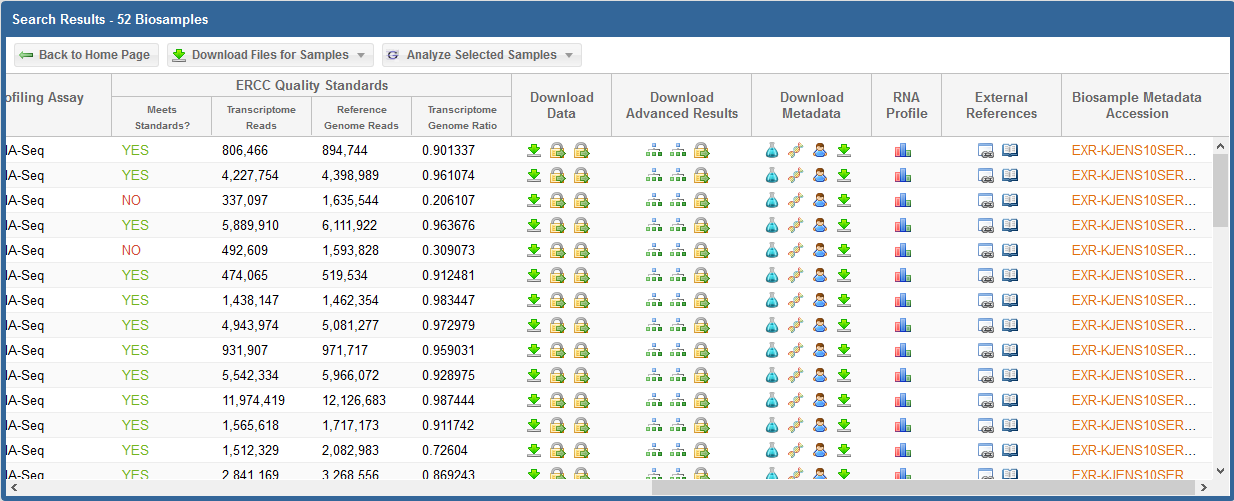
In the first picture above (which displays the first half of the grid), we see each biosample's name as well as some key metadata properties
of each biosample (Condition, Anatomical Location, Biofluid Name, and exRNA Source).
In the second picture above (which displays the second half of the grid), we see the following information and links:
ERCC Quality Standards?
- The grid will display ERCC quality standard metrics for each sample.
The "Meets Standards?" column will clearly indicate whether the sample meets the required quality thresholds: "YES", "NO", or "NA".
A value of "NA" indicates that we are currently reevaluating that sample's quality.
You can view the ERC Consortium QC Standards page to learn more about the QC standards used.
Download Data
- For all profiles, click the icon to download the "core processed results" associated with the sample.
- For RNA-seq profiles, this download will be the exceRpt processed core results archive.
This archive will contain mapped read counts from all three stages of exceRpt (endogenous, exogenous miRNA and rRNA, and exogenous genomes).
- For qPCR profiles, this download will be the qPCR Targets file. The file will contain different miRNA targets and associated Ct values for those targets.
- For RNA-seq profiles, click the
 icon to download the full results (alignments) for the first two stages of exceRpt (endogenous alignment and exogenous miRNA and rRNA alignment).
- For RNA-seq profiles, click the icon to download the original FASTQ source file.
- If you see , this icon means that the data is restricted access and is currently under the protected period (embargo).
The embargo on this dataset will end 12 months after the time the data was submitted to the DCC. View the ERC Consortium Data Access Policy for more details.
- If you see , this icon means that the data is deposited (or will be soon) into a controlled access archive like dbGaP.
You can click the icon under the Actions column to view any available links to controlled access archive(s) that contain data for the relevant biosample.
You can then request access through those external databases.
Download Advanced Results
- For RNA-seq profiles, click the
 icon to download the taxonomy tree (either exogenous ribosomal RNA or exogenous genomic reads) created by exceRpt.
- For RNA-seq profiles, click the icon to download the full results (alignments) for the third stage of exceRpt (exogenous genomic alignment).
- If you see , this icon means that the data is restricted access and is currently under the protected period (embargo).
The embargo on this dataset will end 12 months after the time the data was submitted to the DCC. View the ERC Consortium Data Access Policy for more details.
- If you see , this icon means that the data is deposited (or will be soon) into a controlled access archive like dbGaP.
You can click the icon under the Actions column to view any available links to controlled access archive(s) that contain data for the relevant biosample.
You can then request access through those external databases.
Download Metadata
- Click the
 icon to download the biosample metadata document associated with the biosample.
You can also view the document in GenboreeKB (our UI for viewing metadata) by clicking the biosample's accession ID in the Biosample Metadata Accession column.
- Click the
 icon to download the experiment metadata document associated with the biosample.
- Click the
 icon to download the donor metadata document associated with the biosample.
Actions
- Click the
 icon to view a histogram of read counts mapped to various libraries.
- Click the icon to view information about external databases associated with the biosample.
If the biosample can be found in any external databases (SRA, dbGaP, GEO, etc.), then a link is provided.
If the biosample is still embargoed, then information about the embargo period is displayed, along with a link to the ERCC data access policy.
There are three additional buttons at the top of the grid.
First, the Back to Home Page button will take you back to the exRNA Atlas landing page.
Second, the Download All Samples button will allow you to download result files in bulk.
To learn more about this option, view this tutorial.
Third, the Analyze Selected Samples button will allow you to take samples from the exRNA Atlas and feed them into downstream and comparative analysis tools
present in the Genboree Workbench. To learn more about this option, view this tutorial.
Viewing Atlas Statistics
You can find various Atlas statistics in the Atlas Statistics panel near the bottom of the Atlas homepage. You can reach the Atlas homepage by:
- Clicking the banner at the top of any Atlas page
- Clicking the Home button on the left side of the navigation bar at the top of any Atlas page

On the left side of the panel, you can see various bar charts that describe the data in the Atlas.
- Submitted Samples vs. Biofluid
- Reads Passing Quality Control (QC) vs. Biofluid
- Transcriptome Mapped Reads vs. Biofluid
- Read Mappings vs. RNA Type
On the right side of the panel, you can see a breakdown of how much data has been deposited into the Atlas over various time frames.
Viewing Biosamples in Biosample Partition Grid
As an alternative to the facet search, you can also view all biosamples in one of our biosample partition grids.
We have two different biosample partition grids available: Biofluid vs Condition and Biofluid vs Assay Type.
You can access these grids in two different ways:
First, you can click Select Profiles in the navigation bar and then click Biofluid vs Condition Grid or Biofluid vs Assay Type Grid.
Second, you can use the links on the front page in the Browse exRNA Profiles - Alternative Options panel:
For example, see the Biofluid vs. Condition grid below:
Each cell in this grid indicates the total number of biosamples collected and profiled for exRNAs from a biofluid-condition combination.
If you click the number in a given cell, you will be able to see key metadata about all the biosamples that meet the biofluid-condition criteria given for that cell.
The Biofluid vs. Assay Type grid is very similar except its columns are assay types instead of conditions.
Once you click the number in a given cell, a new grid will be displayed that contains information about associated samples.
In the first picture above (which displays the first half of the grid), we see each biosample's name as well as some key metadata properties
of each biosample (Condition, Anatomical Location, Biofluid Name, and exRNA Source).
In the second picture above (which displays the second half of the grid), we see the following information and links:
ERCC Quality Standards?
- The grid will display ERCC quality standard metrics for each sample.
The "Meets Standards?" column will clearly indicate whether the sample meets the required quality thresholds: "YES", "NO", or "NA".
A value of "NA" indicates that we are currently reevaluating that sample's quality.
You can view the ERC Consortium QC Standards page to learn more about the QC standards used.
Download Data
- For all profiles, click the icon to download the "core processed results" associated with the sample.
- For RNA-seq profiles, this download will be the exceRpt processed core results archive.
This archive will contain mapped read counts from all three stages of exceRpt (endogenous, exogenous miRNA and rRNA, and exogenous genomes).
- For qPCR profiles, this download will be the qPCR Targets file. The file will contain different miRNA targets and associated Ct values for those targets.
- For RNA-seq profiles, click the icon to download the full results (alignments) for the first two stages of exceRpt (endogenous alignment and exogenous miRNA and rRNA alignment).
- For RNA-seq profiles, click the icon to download the original FASTQ source file.
- If you see , this icon means that the data is restricted access and is currently under the protected period (embargo).
The embargo on this dataset will end 12 months after the time the data was submitted to the DCC. View the ERC Consortium Data Access Policy for more details.
- If you see , this icon means that the data is deposited (or will be soon) into a controlled access archive like dbGaP.
You can click the icon under the Actions column to view any available links to controlled access archive(s) that contain data for the relevant biosample.
You can then request access through those external databases.
Download Advanced Results
- For RNA-seq profiles, click the icon to download the taxonomy tree (either exogenous ribosomal RNA or exogenous genomic reads) created by exceRpt.
- For RNA-seq profiles, click the icon to download the full results (alignments) for the third stage of exceRpt (exogenous genomic alignment).
- If you see , this icon means that the data is restricted access and is currently under the protected period (embargo).
The embargo on this dataset will end 12 months after the time the data was submitted to the DCC. View the ERC Consortium Data Access Policy for more details.
- If you see , this icon means that the data is deposited (or will be soon) into a controlled access archive like dbGaP.
You can click the icon under the Actions column to view any available links to controlled access archive(s) that contain data for the relevant biosample.
You can then request access through those external databases.
Download Metadata
- Click the icon to download the biosample metadata document associated with the biosample.
You can also view the document in GenboreeKB (our UI for viewing metadata) by clicking the biosample's accession ID in the Biosample Metadata Accession column.
- Click the icon to download the experiment metadata document associated with the biosample.
- Click the icon to download the donor metadata document associated with the biosample.
- Click the icon to download a file containing all three metadata documents (biosample, donor, and experiment) associated with the biosample.
RNA Profile
- Click the icon to view a histogram of read counts mapped to various libraries.
External References
- Click the icon to view information about external databases associated with the biosample.
If the biosample can be found in any external databases (SRA, dbGaP, GEO, etc.), then a link is provided.
If the biosample is still embargoed, then information about the embargo period is displayed, along with a link to the ERCC data access policy.
- Click the
 icon to open the PubMed page associated with the biosample.
If there is no PubMed page, you will get a pop-up alerting you that no references could be found.
There are three additional buttons at the top of the grid.
First, the Back to Home Page button will take you back to the exRNA Atlas landing page.
Second, the Download All Samples button will allow you to download result files in bulk.
To learn more about this option, view this tutorial.
Third, the Analyze Selected Samples button will allow you to take samples from the exRNA Atlas and feed them into downstream and comparative analysis tools.
To learn more about this option, view this tutorial.
Viewing exRNA Profiling Datasets
All profiles that are submitted to the exRNA Atlas are part of a dataset.
Each dataset is associated with a given study that focuses on some topic (detection of biomarkers associated with gastric cancer, for example).
There are two different ways of viewing datasets on the exRNA Atlas.
Dataset Submissions Table
First, on the Atlas home page, you can find the Dataset Submissions table.
This table provides a summary-level description for each dataset submission to the Atlas.
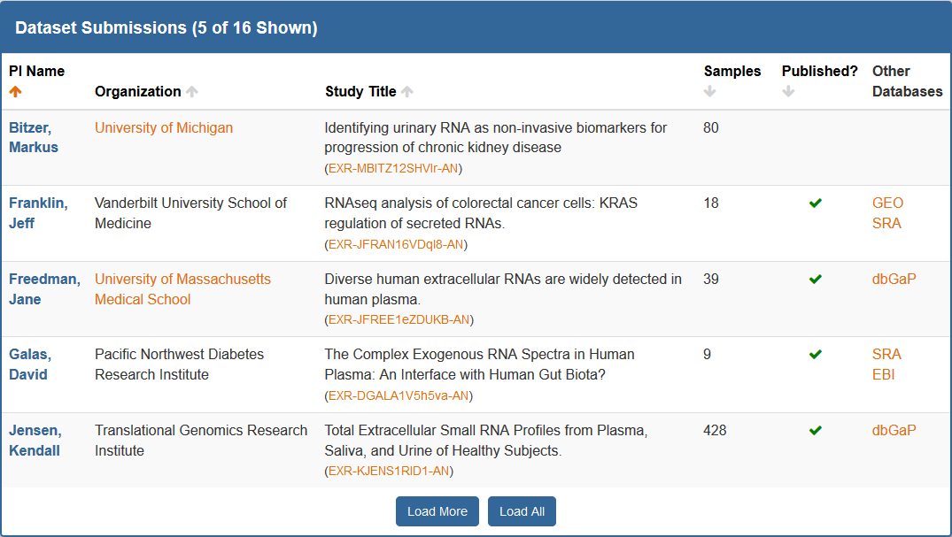
The table, by default, is organized by PI (last) name, but you can sort (ascending or descending) by most of the columns.
Clicking the analysis ID for a given dataset in the Study Title column will take you to its card on the stand-alone Datasets page (described below).
Clicking the green check mark for a given dataset in the Published? column will open the publication associated with that dataset.
Clicking the name of an external database (dbGaP, GEO, SRA) for a given dataset in the Other Databases column will open the associated page for that dataset in the external database.
You can click Load More to load an additional 5 datasets, or click Load All to load all datasets at once.
If you want the table to return to default, you can then click the Return to Default button (only available once you've loaded additional datasets).
Datasets Page
If you want to view datasets in more detail, you can visit the stand-alone Datasets page.
You can reach this page in three different ways:
- Click the Datasets button in the navigation bar at the top of any Atlas page
- Click the exRNA Profiling Datasets link in the Browse exRNA Profiles - Alternative Options panel near the bottom of the Atlas home page
- Click the analysis ID associated with a given dataset in the Dataset Submissions table
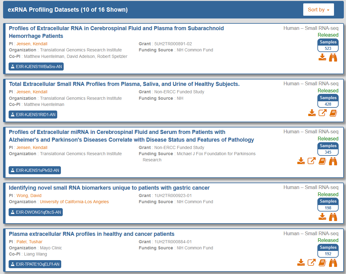
Each card in the layout above contains information about a dataset in the exRNA Atlas:
- The Analysis ID in the lower left corner will open an RNA profile grid for that dataset.
- For RNA-seq profiles, this grid will contain different read counts from various stages of mapping in the exceRpt pipeline.
- For qPCR profiles, this grid will contain sample metadata.
- The Samples badge on the right side will open a grid containing sample metadata for that dataset.
- The
 button will bring up a pop-over window that contains various downloads associated with the dataset.
- The
 button will download a PDF containing different diagnostic plots for the dataset.
- The
 button will download a table of the different raw (not normalized) miRNA read counts for the dataset.
- The
 button will download a text file containing the exogenous genomic taxonomy's cumulative read counts for the dataset.
- The
 button will download a text file containing the exogenous ribosomal RNA taxonomy's cumulative read counts for the dataset.
- The
 button will download an archive containing a large assortment of different summary files for this dataset.
- The
 button will bring up a pop-over window that contains links to external references to the dataset.
- Examples include dbGaP, GEO, BioProject, and ArrayExpress.
- The
 button will bring up a pop-over window that contains links to PubMed articles associated with the dataset.
- The
 button will open up an overview page for the dataset on BioGPS, a gene annotation portal that will allow you to visualize counts for different miRNA species present in the dataset.
Note that not all options will be available for each card.
RNA Profile Grid
By clicking the Analysis ID associated with a given dataset, you can pull up a grid that contains read counts for that dataset.
The grid will also contain various downloads for each sample in the dataset.
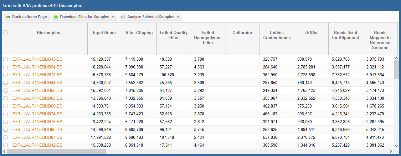
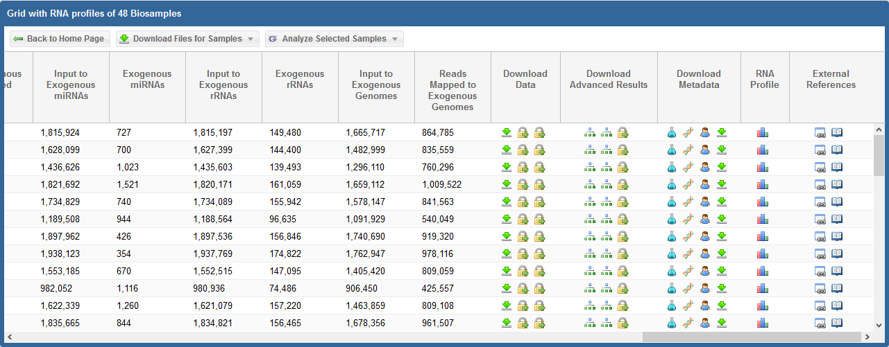
In the first picture above, we see the read counts associated with different exceRpt mapping stages for each sample.
In the second picture above, we see the following information and links:
Download Data
- For all profiles, click the icon to download the "core processed results" associated with the sample.
- For RNA-seq profiles, this download will be the exceRpt processed core results archive.
This archive will contain mapped read counts from all three stages of exceRpt (endogenous, exogenous miRNA and rRNA, and exogenous genomes).
- For qPCR profiles, this download will be the qPCR Targets file. The file will contain different miRNA targets and associated Ct values for those targets.
- For RNA-seq profiles, click the icon to download the full results (alignments) for the first two stages of exceRpt (endogenous alignment and exogenous miRNA and rRNA alignment).
- For RNA-seq profiles, click the icon to download the original FASTQ source file.
- If you see , this icon means that the data is restricted access and is currently under the protected period (embargo).
The embargo on this dataset will end 12 months after the time the data was submitted to the DCC. View the ERC Consortium Data Access Policy for more details.
- If you see , this icon means that the data is deposited (or will be soon) into a controlled access archive like dbGaP.
You can click the icon under the Actions column to view any available links to controlled access archive(s) that contain data for the relevant biosample.
You can then request access through those external databases.
Download Advanced Results
- For RNA-seq profiles, click the icon to download the taxonomy tree (either exogenous ribosomal RNA or exogenous genomic reads) created by exceRpt.
- For RNA-seq profiles, click the icon to download the full results (alignments) for the third stage of exceRpt (exogenous genomic alignment).
- If you see , this icon means that the data is restricted access and is currently under the protected period (embargo).
The embargo on this dataset will end 12 months after the time the data was submitted to the DCC. View the ERC Consortium Data Access Policy for more details.
- If you see , this icon means that the data is deposited (or will be soon) into a controlled access archive like dbGaP.
You can click the icon under the Actions column to view any available links to controlled access archive(s) that contain data for the relevant biosample.
You can then request access through those external databases.
Download Metadata
- Click the icon to download the biosample metadata document associated with the biosample.
You can also view the document in GenboreeKB (our UI for viewing metadata) by clicking the biosample's accession ID in the Biosample Metadata Accession column.
- Click the icon to download the experiment metadata document associated with the biosample.
- Click the icon to download the donor metadata document associated with the biosample.
- Click the icon to download a file containing all three metadata documents (biosample, donor, and experiment) associated with the biosample.
RNA Profile
- Click the icon to view a histogram of read counts mapped to various libraries.
External References
- Click the icon to view information about external databases associated with the biosample.
If the biosample can be found in any external databases (SRA, dbGaP, GEO, etc.), then a link is provided.
If the biosample is still embargoed, then information about the embargo period is displayed, along with a link to the ERCC data access policy.
- Click the icon to open the PubMed page associated with the biosample.
If there is no PubMed page, you will get a pop-up alerting you that no references could be found.
There are three additional buttons at the top of the grid.
First, the Back to Home Page button will take you back to the exRNA Atlas landing page.
Second, the Download All Samples button will allow you to download result files in bulk.
To learn more about this option, view this tutorial.
Third, the Analyze Selected Samples button will allow you to take samples from the exRNA Atlas and feed them into downstream and comparative analysis tools.
To learn more about this option, view this tutorial.
By clicking the Samples badge associated with a given dataset, you can pull up a grid that contains sample metadata for that dataset.
In the first picture above (which displays the first half of the grid), we see each biosample's name as well as some key metadata properties
of each biosample (Condition, Anatomical Location, Biofluid Name, and exRNA Source).
In the second picture above (which displays the second half of the grid), we see the following information and links:
ERCC Quality Standards?
- The grid will display ERCC quality standard metrics for each sample.
The "Meets Standards?" column will clearly indicate whether the sample meets the required quality thresholds: "YES", "NO", or "NA".
A value of "NA" indicates that we are currently reevaluating that sample's quality.
You can view the ERC Consortium QC Standards page to learn more about the QC standards used.
Download Data
- For all profiles, click the icon to download the "core processed results" associated with the sample.
- For RNA-seq profiles, this download will be the exceRpt processed core results archive.
This archive will contain mapped read counts from all three stages of exceRpt (endogenous, exogenous miRNA and rRNA, and exogenous genomes).
- For qPCR profiles, this download will be the qPCR Targets file. The file will contain different miRNA targets and associated Ct values for those targets.
- For RNA-seq profiles, click the icon to download the full results (alignments) for the first two stages of exceRpt (endogenous alignment and exogenous miRNA and rRNA alignment).
- For RNA-seq profiles, click the icon to download the original FASTQ source file.
- If you see , this icon means that the data is restricted access and is currently under the protected period (embargo).
The embargo on this dataset will end 12 months after the time the data was submitted to the DCC. View the ERC Consortium Data Access Policy for more details.
- If you see , this icon means that the data is deposited (or will be soon) into a controlled access archive like dbGaP.
You can click the icon under the Actions column to view any available links to controlled access archive(s) that contain data for the relevant biosample.
You can then request access through those external databases.
Download Advanced Results
- For RNA-seq profiles, click the icon to download the taxonomy tree (either exogenous ribosomal RNA or exogenous genomic reads) created by exceRpt.
- For RNA-seq profiles, click the icon to download the full results (alignments) for the third stage of exceRpt (exogenous genomic alignment).
- If you see , this icon means that the data is restricted access and is currently under the protected period (embargo).
The embargo on this dataset will end 12 months after the time the data was submitted to the DCC. View the ERC Consortium Data Access Policy for more details.
- If you see , this icon means that the data is deposited (or will be soon) into a controlled access archive like dbGaP.
You can click the icon under the Actions column to view any available links to controlled access archive(s) that contain data for the relevant biosample.
You can then request access through those external databases.
Download Metadata
- Click the icon to download the biosample metadata document associated with the biosample.
You can also view the document in GenboreeKB (our UI for viewing metadata) by clicking the biosample's accession ID in the Biosample Metadata Accession column.
- Click the icon to download the experiment metadata document associated with the biosample.
- Click the icon to download the donor metadata document associated with the biosample.
- Click the icon to download a file containing all three metadata documents (biosample, donor, and experiment) associated with the biosample.
RNA Profile
- Click the icon to view a histogram of read counts mapped to various libraries.
External References
- Click the icon to view information about external databases associated with the biosample.
If the biosample can be found in any external databases (SRA, dbGaP, GEO, etc.), then a link is provided.
If the biosample is still embargoed, then information about the embargo period is displayed, along with a link to the ERCC data access policy.
- Click the icon to open the PubMed page associated with the biosample.
If there is no PubMed page, you will get a pop-up alerting you that no references could be found.
There are three additional buttons at the top of the grid.
First, the Back to Home Page button will take you back to the exRNA Atlas landing page.
Second, the Download All Samples button will allow you to download result files in bulk.
To learn more about this option, view this tutorial.
Third, the Analyze Selected Samples button will allow you to take samples from the exRNA Atlas and feed them into downstream and comparative analysis tools.
To learn more about this option, view this tutorial.
Viewing Selected Biosamples in Grid via Faceted Search
It is easy to search for specific types of biosamples via our chart search. There are three different categories which you can use for your search:

You can select exRNA profiles by clicking the slices or names of facets in the charts above.
For example, if I wanted to search for biosamples that were either plasma or serum and were tagged as Alzheimer's disease, I would click the "Plasma", "Serum", and "Alzheimer's" facets.
Then, in order to complete the search, I would click the Search icon in the floating menubar.
This search will create a grid that looks like the following:

This search summary results grid will display key metadata about the relevant biosamples.
- You can download the processed results for a given biosample by clicking its Arrow icon in the Actions column.
- Similarly, you can view the histogram of the read counts mapped to various libraries for a given biosample by clicking
its Bar Chart icon in the Actions column.
- Finally, you can view the full biosample metadata document for a given biosample (in the GenboreeKB UI) by clicking
its Accession ID in the Biosample column.
Tips and tricks:
- If you want to search for all possible facets, you can click the Plus icon below the Search icon to select all facets.
- To deselect any selected facets, click the X icon below the Search icon.
Viewing Selected Biosamples in Grid via Faceted Charts
You can find the faceted search on the Atlas home page. There are many ways to reach it:
- Click the banner at the top of any page on the Atlas
- Click the "Home" button in the navigation bar at the top of any page on the Atlas
- Click Select Profiles in the navigation bar and then click Faceted Charts
It is easy to select specific types of biosamples via our faceted donut charts. There are four different categories which you can use for your selection:
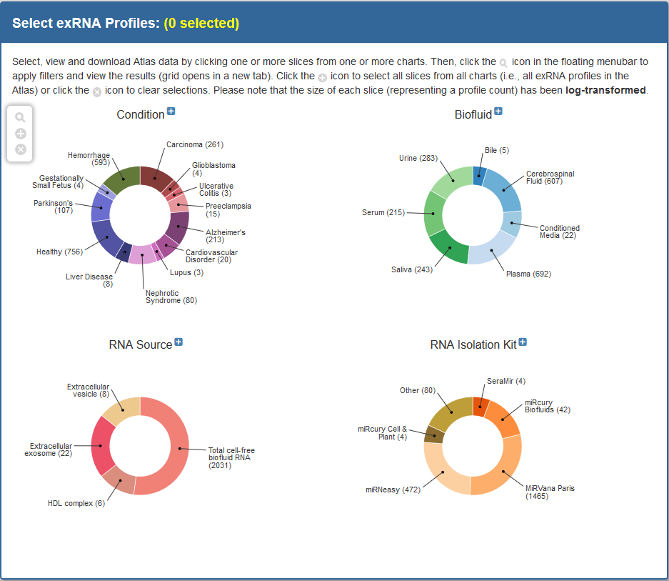
You can select exRNA profiles by clicking the slices or names of facets in the charts.
- If you want to select all possible facets, you can click the
 icon in the floating menubar.
- To deselect any selected facets, click the
 icon in the floating menubar.
- As you select facets, the total number of selected samples will be displayed in red above the charts.
Example: If I wanted to select biosamples that were either plasma or serum and were tagged as Alzheimer's disease, I would click the "Alzheimer's", "Plasma", and "Serum" facets.
Because 52 samples (as of July 28th, 2016) qualify for these facets, (52 selected) will be displayed in yellow above the faceted charts.
Then, in order to generate my grid, I would click the  icon in the floating menubar.
Clicking this icon will create a grid that looks like the following (split up into two separate pictures, each depicting half of the grid):
In the first picture above (which displays the first half of the grid), we see each biosample's name as well as some key metadata properties
of each biosample (Condition, Anatomical Location, Biofluid Name, and exRNA Source).
In the second picture above (which displays the second half of the grid), we see the following information and links:
ERCC Quality Standards?
- The grid will display ERCC quality standard metrics for each sample.
The "Meets Standards?" column will clearly indicate whether the sample meets the required quality thresholds: "YES", "NO", or "NA".
A value of "NA" indicates that we are currently reevaluating that sample's quality.
You can view the ERC Consortium QC Standards page to learn more about the QC standards used.
Download Data
- For all profiles, click the icon to download the "core processed results" associated with the sample.
- For RNA-seq profiles, this download will be the exceRpt processed core results archive.
This archive will contain mapped read counts from all three stages of exceRpt (endogenous, exogenous miRNA and rRNA, and exogenous genomes).
- For qPCR profiles, this download will be the qPCR Targets file. The file will contain different miRNA targets and associated Ct values for those targets.
- For RNA-seq profiles, click the icon to download the full results (alignments) for the first two stages of exceRpt (endogenous alignment and exogenous miRNA and rRNA alignment).
- For RNA-seq profiles, click the icon to download the original FASTQ source file.
- If you see , this icon means that the data is restricted access and is currently under the protected period (embargo).
The embargo on this dataset will end 12 months after the time the data was submitted to the DCC. View the ERC Consortium Data Access Policy for more details.
- If you see , this icon means that the data is deposited (or will be soon) into a controlled access archive like dbGaP.
You can click the icon under the Actions column to view any available links to controlled access archive(s) that contain data for the relevant biosample.
You can then request access through those external databases.
Download Advanced Results
- For RNA-seq profiles, click the icon to download the taxonomy tree (either exogenous ribosomal RNA or exogenous genomic reads) created by exceRpt.
- For RNA-seq profiles, click the icon to download the full results (alignments) for the third stage of exceRpt (exogenous genomic alignment).
- If you see , this icon means that the data is restricted access and is currently under the protected period (embargo).
The embargo on this dataset will end 12 months after the time the data was submitted to the DCC. View the ERC Consortium Data Access Policy for more details.
- If you see , this icon means that the data is deposited (or will be soon) into a controlled access archive like dbGaP.
You can click the icon under the Actions column to view any available links to controlled access archive(s) that contain data for the relevant biosample.
You can then request access through those external databases.
Download Metadata
- Click the icon to download the biosample metadata document associated with the biosample.
You can also view the document in GenboreeKB (our UI for viewing metadata) by clicking the biosample's accession ID in the Biosample Metadata Accession column.
- Click the icon to download the experiment metadata document associated with the biosample.
- Click the icon to download the donor metadata document associated with the biosample.
- Click the icon to download a file containing all three metadata documents (biosample, donor, and experiment) associated with the biosample.
RNA Profile
- Click the icon to view a histogram of read counts mapped to various libraries.
External References
- Click the icon to view information about external databases associated with the biosample.
If the biosample can be found in any external databases (SRA, dbGaP, GEO, etc.), then a link is provided.
If the biosample is still embargoed, then information about the embargo period is displayed, along with a link to the ERCC data access policy.
- Click the icon to open the PubMed page associated with the biosample.
If there is no PubMed page, you will get a pop-up alerting you that no references could be found.
There are three additional buttons at the top of the grid.
First, the Back to Home Page button will take you back to the exRNA Atlas landing page.
Second, the Download All Samples button will allow you to download result files in bulk.
To learn more about this option, view this tutorial.
Third, the Analyze Selected Samples button will allow you to take samples from the exRNA Atlas and feed them into downstream and comparative analysis tools.
To learn more about this option, view this tutorial.
Viewing Selected Biosamples in Grid via Faceted Search
You can find the faceted search on the Atlas home page. There are many ways to reach it:
- Click the banner at the top of any page on the Atlas
- Click the "Home" button in the navigation bar at the top of any page on the Atlas
- Click Select Profiles in the navigation bar and then click Faceted Charts
It is easy to select specific types of biosamples via our faceted donut charts. There are four different categories which you can use for your selection:
You can select exRNA profiles by clicking the slices or names of facets in the charts.
- If you want to select all possible facets, you can click the icon in the floating menubar.
- To deselect any selected facets, click the icon in the floating menubar.
- As you select facets, the total number of selected samples will be displayed in red above the charts.
Example: If I wanted to select biosamples that were either plasma or serum and were tagged as Alzheimer's disease, I would click the "Alzheimer's", "Plasma", and "Serum" facets.
Because 52 samples (as of July 28th, 2016) qualify for these facets, (52 selected) will be displayed in yellow above the faceted charts.
Then, in order to generate my grid, I would click the icon in the floating menubar.
Clicking this icon will create a grid that looks like the following (split up into two separate pictures, each depicting half of the grid):
In the first picture above (which displays the first half of the grid), we see each biosample's name as well as some key metadata properties
of each biosample (Condition, Anatomical Location, Biofluid Name, and exRNA Source).
In the second picture above (which displays the second half of the grid), we see the following information and links:
ERCC Quality Standards?
- The grid will display ERCC quality standard metrics for each sample.
The "Meets Standards?" column will clearly indicate whether the sample meets the required quality thresholds: "YES", "NO", or "NA".
A value of "NA" indicates that we are currently reevaluating that sample's quality.
You can view the ERC Consortium QC Standards page to learn more about the QC standards used.
Download Data
- For all profiles, click the icon to download the "core processed results" associated with the sample.
- For RNA-seq profiles, this download will be the exceRpt processed core results archive.
This archive will contain mapped read counts from all three stages of exceRpt (endogenous, exogenous miRNA and rRNA, and exogenous genomes).
- For qPCR profiles, this download will be the qPCR Targets file. The file will contain different miRNA targets and associated Ct values for those targets.
- For RNA-seq profiles, click the icon to download the full results (alignments) for the first two stages of exceRpt (endogenous alignment and exogenous miRNA and rRNA alignment).
- For RNA-seq profiles, click the icon to download the original FASTQ source file.
- If you see , this icon means that the data is restricted access and is currently under the protected period (embargo).
The embargo on this dataset will end 12 months after the time the data was submitted to the DCC. View the ERC Consortium Data Access Policy for more details.
- If you see , this icon means that the data is deposited (or will be soon) into a controlled access archive like dbGaP.
You can click the icon under the Actions column to view any available links to controlled access archive(s) that contain data for the relevant biosample.
You can then request access through those external databases.
Download Advanced Results
- For RNA-seq profiles, click the icon to download the taxonomy tree (either exogenous ribosomal RNA or exogenous genomic reads) created by exceRpt.
- For RNA-seq profiles, click the icon to download the full results (alignments) for the third stage of exceRpt (exogenous genomic alignment).
- If you see , this icon means that the data is restricted access and is currently under the protected period (embargo).
The embargo on this dataset will end 12 months after the time the data was submitted to the DCC. View the ERC Consortium Data Access Policy for more details.
- If you see , this icon means that the data is deposited (or will be soon) into a controlled access archive like dbGaP.
You can click the icon under the Actions column to view any available links to controlled access archive(s) that contain data for the relevant biosample.
You can then request access through those external databases.
Download Metadata
- Click the icon to download the biosample metadata document associated with the biosample.
You can also view the document in GenboreeKB (our UI for viewing metadata) by clicking the biosample's accession ID in the Biosample Metadata Accession column.
- Click the icon to download the experiment metadata document associated with the biosample.
- Click the icon to download the donor metadata document associated with the biosample.
Actions
- Click the icon to view a histogram of read counts mapped to various libraries.
- Click the icon to view information about external databases associated with the biosample.
If the biosample can be found in any external databases (SRA, dbGaP, GEO, etc.), then a link is provided.
If the biosample is still embargoed, then information about the embargo period is displayed, along with a link to the ERCC data access policy.
There are three additional buttons at the top of the grid.
First, the Back to Home Page button will take you back to the exRNA Atlas landing page.
Second, the Download All Samples button will allow you to download result files in bulk.
To learn more about this option, view this tutorial.
Third, the Analyze Selected Samples button will allow you to take samples from the exRNA Atlas and feed them into downstream and comparative analysis tools
present in the Genboree Workbench. To learn more about this option, view this tutorial.
Viewing Selected Biosamples in Grid via Linear Tree
You can use our dendrogram-like partition diagram ("linear tree") to interactively drill down into different subsets of biosamples.
There are two ways of reaching the linear tree page:
- Click the Select Profiles button in the navigation bar and then click the Linear Tree Drill-Down button.
- Go to the Atlas homepage and click the Linear Tree Drill-Down link in the Browse exRNA Profiles - Alternative Options panel.
After you open the linear tree drill-down page, you will see a diagram like the following:
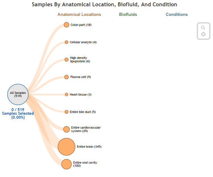
Click on a collapsed node to "drill down" along its path in the Anatomical Locations » Biofluids » Conditions facet sequence.
- Click on an expanded node to collapse it.
- Reset/clear your active path using the icon in the floating menubar.
Your selected path is always clearly highlighted:
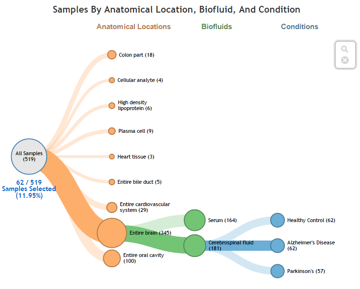
Clicking the icon in the floating menubar will open the search results for your particular drill-down path (split up into two separate pictures, each depicting half of the grid):
In the first picture above (which displays the first half of the grid), we see each biosample's name as well as some key metadata properties
of each biosample (Condition, Anatomical Location, Biofluid Name, and exRNA Source).
In the second picture above (which displays the second half of the grid), we see the following information and links:
ERCC Quality Standards?
- The grid will display ERCC quality standard metrics for each sample.
The "Meets Standards?" column will clearly indicate whether the sample meets the required quality thresholds: "YES", "NO", or "NA".
A value of "NA" indicates that we are currently reevaluating that sample's quality.
You can view the ERC Consortium QC Standards page to learn more about the QC standards used.
Download Data
- For all profiles, click the icon to download the "core processed results" associated with the sample.
- For RNA-seq profiles, this download will be the exceRpt processed core results archive.
This archive will contain mapped read counts from all three stages of exceRpt (endogenous, exogenous miRNA and rRNA, and exogenous genomes).
- For qPCR profiles, this download will be the qPCR Targets file. The file will contain different miRNA targets and associated Ct values for those targets.
- For RNA-seq profiles, click the icon to download the full results (alignments) for the first two stages of exceRpt (endogenous alignment and exogenous miRNA and rRNA alignment).
- For RNA-seq profiles, click the icon to download the original FASTQ source file.
- If you see , this icon means that the data is restricted access and is currently under the protected period (embargo).
The embargo on this dataset will end 12 months after the time the data was submitted to the DCC. View the ERC Consortium Data Access Policy for more details.
- If you see , this icon means that the data is deposited (or will be soon) into a controlled access archive like dbGaP.
You can click the icon under the Actions column to view any available links to controlled access archive(s) that contain data for the relevant biosample.
You can then request access through those external databases.
Download Advanced Results
- For RNA-seq profiles, click the icon to download the taxonomy tree (either exogenous ribosomal RNA or exogenous genomic reads) created by exceRpt.
- For RNA-seq profiles, click the icon to download the full results (alignments) for the third stage of exceRpt (exogenous genomic alignment).
- If you see , this icon means that the data is restricted access and is currently under the protected period (embargo).
The embargo on this dataset will end 12 months after the time the data was submitted to the DCC. View the ERC Consortium Data Access Policy for more details.
- If you see , this icon means that the data is deposited (or will be soon) into a controlled access archive like dbGaP.
You can click the icon under the Actions column to view any available links to controlled access archive(s) that contain data for the relevant biosample.
You can then request access through those external databases.
Download Metadata
- Click the icon to download the biosample metadata document associated with the biosample.
You can also view the document in GenboreeKB (our UI for viewing metadata) by clicking the biosample's accession ID in the Biosample Metadata Accession column.
- Click the icon to download the experiment metadata document associated with the biosample.
- Click the icon to download the donor metadata document associated with the biosample.
- Click the icon to download a file containing all three metadata documents (biosample, donor, and experiment) associated with the biosample.
RNA Profile
- Click the icon to view a histogram of read counts mapped to various libraries.
External References
- Click the icon to view information about external databases associated with the biosample.
If the biosample can be found in any external databases (SRA, dbGaP, GEO, etc.), then a link is provided.
If the biosample is still embargoed, then information about the embargo period is displayed, along with a link to the ERCC data access policy.
- Click the icon to open the PubMed page associated with the biosample.
If there is no PubMed page, you will get a pop-up alerting you that no references could be found.
There are three additional buttons at the top of the grid.
First, the Back to Home Page button will take you back to the exRNA Atlas landing page.
Second, the Download All Samples button will allow you to download result files in bulk.
To learn more about this option, view this tutorial.
Third, the Analyze Selected Samples button will allow you to take samples from the exRNA Atlas and feed them into downstream and comparative analysis tools.
To learn more about this option, view this tutorial.
N/A
Viewing Summary Barcharts of exRNA Profiling Datasets
On the main Atlas landing page, there are several different barcharts in the Atlas Statistics section that summarize the exRNA profiling datasets held within the Atlas.
Different summary metrics include:
- Submitted Samples vs Biofluid
- Reads Passing Quality Control (QC) vs Biofluid
- Transcriptome Mapped Reads vs Biofluid
- Read Mappings vs RNA Type
An example barchart can be found below:

Hovering over any of the bars will display the percentage (y-axis) associated with that bar:

Viewing Summary Bar Charts of exRNA Profiling Datasets
On the main Atlas landing page, there are several different bar charts in the Atlas Statistics section that summarize the exRNA profiling datasets held within the Atlas.
Different summary metrics include:
- Submitted Samples vs Biofluid
- Reads Passing Quality Control (QC) vs Biofluid
- Transcriptome Mapped Reads vs Biofluid
- Read Mappings vs RNA Type
An example bar chart can be found below:
Hovering over any of the bars will display the percentage (y-axis) associated with that bar:
Viewing Summary Bar Graphs of exRNA Profiling Datasets
On the main Atlas landing page, there are several different bar graphs in the Atlas Statistics section that summarize the exRNA profiling datasets held within the Atlas.
Different summary metrics include:
- Submitted Samples vs Biofluid
- Reads Passing Quality Control (QC) vs Biofluid
- Transcriptome Mapped Reads vs Biofluid
- Read Mappings vs RNA Type
An example bar graph can be found below:
Hovering over any of the bars will display the percentage (y-axis) associated with that bar:
Viewing Summary Grid of DCC Submissions
The DCC Submission Summary table displays usage of exRNA profiling data analysis tools by both ERC consortium members as well as other members of the scientific community.
In order to view the grid, click the relevant thumbnail on the main Atlas page:
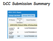
When you click this thumbnail, you will see a grid like the following:
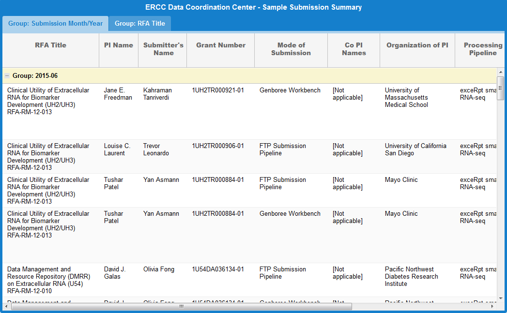
This grid, by default, groups submissions by submission month / year.
However, if you want to group submissions by RFA Title, you can click the Group: RFA Title tab at the top of the grid.
Viewing exRNA Profiling Datasets
All profiles that are submitted to the exRNA Atlas are part of a dataset.
Each dataset is associated with a given study that focuses on some topic (detection of biomarkers associated with gastric cancer, for example).
There are two different ways of viewing datasets on the exRNA Atlas.
Dataset Submissions Table
First, on the Atlas home page, you can find the Dataset Submissions table.
This table provides a summary-level description for each dataset submission to the Atlas.
The table, by default, is organized by PI (last) name, but you can sort (ascending or descending) by most of the columns.
Clicking the analysis ID for a given dataset in the Study Title column will take you to its card on the stand-alone Datasets page (described below).
Clicking the green check mark for a given dataset in the Published? column will open the publication associated with that dataset.
Clicking the name of an external database (dbGaP, GEO, SRA) for a given dataset in the Other Databases column will open the associated page for that dataset in the external database.
You can click Load More to load an additional 5 datasets, or click Load All to load all datasets at once.
If you want the table to return to default, you can then click the Return to Default button (only available once you've loaded additional datasets).
Datasets Page
If you want to view datasets in more detail, you can visit the stand-alone Datasets page.
You can reach this page in three different ways:
- Click the Datasets button in the navigation bar at the top of any Atlas page
- Click the exRNA Profiling Datasets link in the Browse exRNA Profiles - Alternative Options panel near the bottom of the Atlas home page
- Click the analysis ID associated with a given dataset in the Dataset Submissions table
Each card in the layout above contains information about a dataset in the exRNA Atlas:
- The Analysis ID in the lower left corner will open an RNA profile grid for that dataset.
- For RNA-seq profiles, this grid will contain different read counts from various stages of mapping in the exceRpt pipeline.
- For qPCR profiles, this grid will contain sample metadata.
- The Samples badge on the right side will open a grid containing sample metadata for that dataset.
- The button will bring up a pop-over window that contains various downloads associated with the dataset.
- The button will download a PDF containing different diagnostic plots for the dataset.
- The button will download a table of the different raw (not normalized) miRNA read counts for the dataset.
- The button will download a text file containing the exogenous genomic taxonomy's cumulative read counts for the dataset.
- The button will download a text file containing the exogenous ribosomal RNA taxonomy's cumulative read counts for the dataset.
- The button will download an archive containing a large assortment of different summary files for this dataset.
- The button will bring up a pop-over window that contains links to external references to the dataset.
- Examples include dbGaP, GEO, BioProject, and ArrayExpress.
- The button will bring up a pop-over window that contains links to PubMed articles associated with the dataset.
- The button will open up an overview page for the dataset on BioGPS, a gene annotation portal that will allow you to visualize counts for different miRNA species present in the dataset.
Note that not all options will be available for each card.
RNA Profile Grid
By clicking the Analysis ID associated with a given dataset, you can pull up a grid that contains read counts for that dataset.
The grid will also contain various downloads for each sample in the dataset.
In the first picture above, we see the read counts associated with different exceRpt mapping stages for each sample.
In the second picture above, we see the following information and links:
Download Data
- For all profiles, click the icon to download the "core processed results" associated with the sample.
- For RNA-seq profiles, this download will be the exceRpt processed core results archive.
This archive will contain mapped read counts from all three stages of exceRpt (endogenous, exogenous miRNA and rRNA, and exogenous genomes).
- For qPCR profiles, this download will be the qPCR Targets file. The file will contain different miRNA targets and associated Ct values for those targets.
- For RNA-seq profiles, click the icon to download the full results (alignments) for the first two stages of exceRpt (endogenous alignment and exogenous miRNA and rRNA alignment).
- For RNA-seq profiles, click the icon to download the original FASTQ source file.
- If you see , this icon means that the data is restricted access and is currently under the protected period (embargo).
The embargo on this dataset will end 12 months after the time the data was submitted to the DCC. View the ERC Consortium Data Access Policy for more details.
- If you see , this icon means that the data is deposited (or will be soon) into a controlled access archive like dbGaP.
You can click the icon under the Actions column to view any available links to controlled access archive(s) that contain data for the relevant biosample.
You can then request access through those external databases.
Download Advanced Results
- For RNA-seq profiles, click the icon to download the taxonomy tree (either exogenous ribosomal RNA or exogenous genomic reads) created by exceRpt.
- For RNA-seq profiles, click the icon to download the full results (alignments) for the third stage of exceRpt (exogenous genomic alignment).
- If you see , this icon means that the data is restricted access and is currently under the protected period (embargo).
The embargo on this dataset will end 12 months after the time the data was submitted to the DCC. View the ERC Consortium Data Access Policy for more details.
- If you see , this icon means that the data is deposited (or will be soon) into a controlled access archive like dbGaP.
You can click the icon under the Actions column to view any available links to controlled access archive(s) that contain data for the relevant biosample.
You can then request access through those external databases.
Download Metadata
- Click the icon to download the biosample metadata document associated with the biosample.
You can also view the document in GenboreeKB (our UI for viewing metadata) by clicking the biosample's accession ID in the Biosample Metadata Accession column.
- Click the icon to download the experiment metadata document associated with the biosample.
- Click the icon to download the donor metadata document associated with the biosample.
- Click the icon to download a file containing all three metadata documents (biosample, donor, and experiment) associated with the biosample.
RNA Profile
- Click the icon to view a histogram of read counts mapped to various libraries.
External References
- Click the icon to view information about external databases associated with the biosample.
If the biosample can be found in any external databases (SRA, dbGaP, GEO, etc.), then a link is provided.
If the biosample is still embargoed, then information about the embargo period is displayed, along with a link to the ERCC data access policy.
- Click the icon to open the PubMed page associated with the biosample.
If there is no PubMed page, you will get a pop-up alerting you that no references could be found.
There are three additional buttons at the top of the grid.
First, the Back to Home Page button will take you back to the exRNA Atlas landing page.
Second, the Download All Samples button will allow you to download result files in bulk.
To learn more about this option, view this tutorial.
Third, the Analyze Selected Samples button will allow you to take samples from the exRNA Atlas and feed them into downstream and comparative analysis tools.
To learn more about this option, view this tutorial.
By clicking the Samples badge associated with a given dataset, you can pull up a grid that contains sample metadata for that dataset.
In the first picture above (which displays the first half of the grid), we see each biosample's name as well as some key metadata properties
of each biosample (Condition, Anatomical Location, Biofluid Name, and exRNA Source).
In the second picture above (which displays the second half of the grid), we see the following information and links:
ERCC Quality Standards?
- The grid will display ERCC quality standard metrics for each sample.
The "Meets Standards?" column will clearly indicate whether the sample meets the required quality thresholds: "YES", "NO", or "NA".
A value of "NA" indicates that we are currently reevaluating that sample's quality.
You can view the ERC Consortium QC Standards page to learn more about the QC standards used.
Download Data
- For all profiles, click the icon to download the "core processed results" associated with the sample.
- For RNA-seq profiles, this download will be the exceRpt processed core results archive.
This archive will contain mapped read counts from all three stages of exceRpt (endogenous, exogenous miRNA and rRNA, and exogenous genomes).
- For qPCR profiles, this download will be the qPCR Targets file. The file will contain different miRNA targets and associated Ct values for those targets.
- For RNA-seq profiles, click the icon to download the full results (alignments) for the first two stages of exceRpt (endogenous alignment and exogenous miRNA and rRNA alignment).
- For RNA-seq profiles, click the icon to download the original FASTQ source file.
- If you see , this icon means that the data is restricted access and is currently under the protected period (embargo).
The embargo on this dataset will end 12 months after the time the data was submitted to the DCC. View the ERC Consortium Data Access Policy for more details.
- If you see , this icon means that the data is deposited (or will be soon) into a controlled access archive like dbGaP.
You can click the icon under the Actions column to view any available links to controlled access archive(s) that contain data for the relevant biosample.
You can then request access through those external databases.
Download Advanced Results
- For RNA-seq profiles, click the icon to download the taxonomy tree (either exogenous ribosomal RNA or exogenous genomic reads) created by exceRpt.
- For RNA-seq profiles, click the icon to download the full results (alignments) for the third stage of exceRpt (exogenous genomic alignment).
- If you see , this icon means that the data is restricted access and is currently under the protected period (embargo).
The embargo on this dataset will end 12 months after the time the data was submitted to the DCC. View the ERC Consortium Data Access Policy for more details.
- If you see , this icon means that the data is deposited (or will be soon) into a controlled access archive like dbGaP.
You can click the icon under the Actions column to view any available links to controlled access archive(s) that contain data for the relevant biosample.
You can then request access through those external databases.
Download Metadata
- Click the icon to download the biosample metadata document associated with the biosample.
You can also view the document in GenboreeKB (our UI for viewing metadata) by clicking the biosample's accession ID in the Biosample Metadata Accession column.
- Click the icon to download the experiment metadata document associated with the biosample.
- Click the icon to download the donor metadata document associated with the biosample.
- Click the icon to download a file containing all three metadata documents (biosample, donor, and experiment) associated with the biosample.
RNA Profile
- Click the icon to view a histogram of read counts mapped to various libraries.
External References
- Click the icon to view information about external databases associated with the biosample.
If the biosample can be found in any external databases (SRA, dbGaP, GEO, etc.), then a link is provided.
If the biosample is still embargoed, then information about the embargo period is displayed, along with a link to the ERCC data access policy.
- Click the icon to open the PubMed page associated with the biosample.
If there is no PubMed page, you will get a pop-up alerting you that no references could be found.
There are three additional buttons at the top of the grid.
First, the Back to Home Page button will take you back to the exRNA Atlas landing page.
Second, the Download All Samples button will allow you to download result files in bulk.
To learn more about this option, view this tutorial.
Third, the Analyze Selected Samples button will allow you to take samples from the exRNA Atlas and feed them into downstream and comparative analysis tools.
To learn more about this option, view this tutorial.
Viewing Your Results
After you upload your files to our FTP server, we will process your files automatically.
- Processing your files can take anywhere from a few hours to a few days (depending on the size of your submission).
- You will receive a variety of emails while we're processing your files, and an "ERCC Final Processing" email will indicate that your processing is complete.
- It is likely that your initial submission will fail for some reason (invalid metadata, some issue with your manifest file, etc.). This is totally normal!
Read through our Troubleshooting guide if you receive a failure email.
- You can then view your data results and metadata results.
- Your data results will be located on the FTP server (and you will be able to access them through the Genboree Workbench).
- Your metadata results will be located on the exRNA GenboreeKB.
- Both data and metadata will also be available through the private, ERCC-only exRNA Atlas.
Locating Your Data Results on the Genboree Workbench
- Log onto the Genboree Workbench using your Genboree user name and password.
- Read the e-mail you received - it contains a handy ASCII graphic that will illustrate where to find your files.
- Your results will be organized into individual folders (by sample).
- You can find post-processing files generated by the exceRpt Post-Processing tool in the "postProcessedResults_v4.6.3" folder.
Important Notes:
- You will not be able to access your original FTP submission (manifest / metadata archive / data archive) via the Genboree Workbench.
- Anyone who wants access to the data results will need to be a member of the "exRNA Metadata Standards" Group on the Genboree Workbench.
Locating Your Data Results on the FTP Server
Preliminary Steps for New Users
- In order to view your data results on the FTP server, you will need to send the exRNA Team an email requesting FTP access to the private Atlas Virtual FTP Area.
- You should also include your Genboree username, as well as any other Genboree usernames that might need access to the files via FTP client.
- If new users come along later and need access, that's OK - we can always add them later.
- Once we have given you access to see the private Atlas Virtual FTP Area on your FTP client, you will be able to see all submissions to the Atlas.
Locating Your Result Files
- After we have given you access to the private Atlas Virtual FTP Area, log into our FTP server at ftps.genboree.org with your Genboree username and password.
- When you log in, you should see a directory named genboree:genboree.org. Follow the path below to find your results:
- /genboree:genboree.org/exRNA_Metadata_Standards/exRNA_Repository_-_hg19/exRNA-atlas/exceRptPipeline_v4.6.2
- Your results will be listed under the analysis name you gave in the manifest file (or with a generic, time-stamped name if you didn't give an analysis name).
- If your samples fall under a different genome (mm10, for example), then the path above will have that genome instead of hg19.
Locating Your Original Submission
- You will be able to find your original submission (manifest file / metadata archive / data archive) by going to your lab's shared directory (exrna-[pi ID]).
- Then, navigate to the finished directory. Your files will be located in one of the subdirectories (specified in your ERCC Final Processing email).
Understanding Your Data Results
- Regardless of whether you access your data results by Genboree Workbench or FTP client, there will be a number of folders located inside the folder with your Analysis name.
- Each subfolder, except two, corresponds to a sample that you submitted for analysis.
- One subfolder, named postProcessedResults_v4.6.3, contains post-processing results created by the exceRpt small RNA-seq Post-Processing tool.
- This tool merges information from all of the different samples and creates useful visualizations (tables, plots).
- To learn more about this tool, view the exceRpt Tutorial Page.
- The other subfolder, named metadataFiles, contains copies of the metadata files submitted to the exRNA GenboreeKB for storage.
- These files are not the same as the metadata documents you submitted, for the most part - they have been edited and added onto by the pipeline.
- Within each sample's folder, there will be the results associated with that sample.
- To learn more about how to interpret your results, view the exceRpt Data Analysis page.
- Click the Job document link given to you in your email. This document will contain all of the different document IDs associated with your job.
- Click a given ID to be taken to that document. You can open the document in your current tab or in a new tab.
- You can learn more about navigating the exRNA Genboree KB UI in GenboreeKB exRNA Metadata Tracking System - Navigating the Metadata UI.
Copying Your Submission to the Public Atlas
- By default, your submission through the FTP Pipeline will be uploaded to the private, ERCC-only Atlas.
- If you would like your submission to be available on the public Atlas (so that non-ERCC members can see it),
please email Emily requesting that your submission be copied to the public Atlas.
- Once the submission has been copied to the public Atlas, you will be able to find associated data and metadata files
on the Genboree Workbench / FTP Server / GenboreeKB in the following locations:
- Genboree Workbench: "Extracellular RNA Atlas" Group -> [Database listed in your manifest file] Database -> Files -> "exRNA-Atlas" -> exceRptPipeline_v4.3.3 -> [Analysis name]
- FTP Server: /genboree:genboree.org/Extracellular_RNA_Atlas/exRNA_Repository_-_hg19/exRNA-atlas/exceRptPipeline_v4.3.3 (please contact us if you don't have access)
- GenboreeKB: "Extracellular RNA Atlas" project. More info can be found here: GenboreeKB exRNA Metadata Tracking System - Navigating the Metadata UI.