| HELP TOPIC: “10. Circos Interface” |
On This Page:
- 10.1 Circos
- 10.2 Entry Points
- 10.2.1 Global Entry Point Properties
- 10.2.2 Entry Points List
- 10.2.3 Manually Specifying Entry Points
- 10.2.4 Individual Entry Point Properties
- 10.2.5 Entry Point Scales
- 10.2.6 Entry Point Breaks
- 10.3 Specifying Ideogram Properties
- 10.4 Tick Marks
- 10.5 Annotation Tracks
- 10.5.1 Track Types and Options
- 10.5.2 Adding Annotation Tracks
- 10.5.3 Updating Annotation Tracks
- 10.5.4 Removing Annotation Tracks
- 10.5.5 Annotation Filtering Rules
- 10.6 Submitting a Circos Job
Circos is a visualization tool created by Martin Krzywinski from the Michael Smith Genome Sciences Centre of Canada. Circos is a powerful command line tool that is particularly well suited for visualizing comparative genomics data, such as alignments, conservation and duplication events. Circos also supports drawing generalized 2D data in the form of line plots, scatter plots, heatmaps and histograms. Unlike other visualization tools, Circos conveys information by drawing circular ideograms, which makes it extremely valuable for displaying intra- and inter-chromosomal relationships. Circos is similar to other circular visualization tools such as chromowheel or genopix. However, Circos' extremely flexible engine allows the user significant control and customization opportunities that can result in publication-quality, aesthetically pleasing images.
Circos has an extensive variety of tutorials and tutorial images which provide information regarding the capabilities of Circos and the available options for creating images. Circos has also been published: Circos: an Information Aesthetic for Comparative Genomics.
The Circos User Interface (UI) was created to provide users with a simple way to use this powerful command-line tool. Currently, the provided Circos UI supports options for the version 0.51-1 release. Circos is an extremely powerful and flexible tool that can respond to a large number of options and customizations. While the available options in the UI allow a user a high level of control over the resulting image, further options have been left out for simplicity. Please keep in mind that while visiting the Circos webpage and viewing the available tutorials, not all options discussed will be available in the interface. However, after running Circos, you will be able to download all necessary configuration files for your Circos run. If you would like to install Circos on your local machine, you can alter your downloaded configuration file to explore those other options.
The Circos UI provides a wizard-like interface for configuring a run of Circos. Each tab can be traversed in order by clicking the Next Step and Previous Step buttons. However visiting each tab is not required to configure Circos. If you are familiar with the Circos UI and know exactly which tab to visit to customize your desired option you can go directly to the tab by clicking on the tab title.
On the Select Entry Points tab, a user can specify which entry points should be drawn in the image and also modify the appearance of entry points. Circos images comprise a circular representation of entry points with data tracks that can be drawn inside or outside of the circular composition. The symbolic representation of the entry points are called ideograms. In the Genboree context, a Circos ideogram can be thought of as the physical representation of an entry point.
NOTE: At least one entry point must be selected for drawing
In the Specification for All Entry Points section, the user can set properites that will be applied to all entry points that are drawn in the image. The options that can be collectively specified for all entry points are describe below.
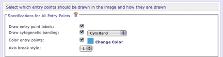
Enable/disable the drawing of entry point labels. Entry point labels alert the user to which entry point they are viewing in the resulting image.
Cytogenetic bands can be drawn on top of the entry points. Upon enabling cytogenetic banding, a list of all annotation tracks will appear. Select the annotation track that contains the banding information
Specify a color to fill each entry point. After enabling coloring, a color selection widget will appear.
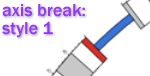
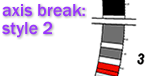
Specify the visual style to be used when indicating sequence breaks in the ideogram
-
Style 1:
-
Style 2:
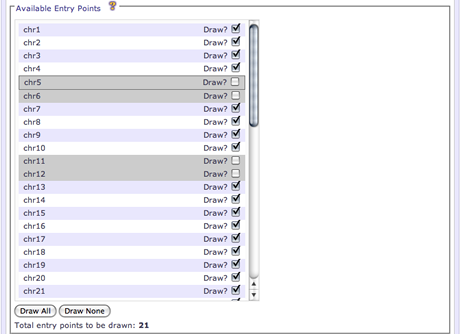
When there is a reasonably small number of entry points available (<100), the UI will display the available entry points as a list. An entry point can be enabled/disabled for drawing by checking the Draw check-box next to the entry point name. Disabled entry points will have a gray background. By default, all *_random entry points will not be drawn.
In this selection mode, Draw All and Draw None buttons are available to quickly select all or clear all entry points for drawing, respectively.
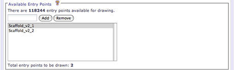
When the available entry points in a database is relatively large (>100), the UI will require the user to manually specify the entry points to be drawn by name. The UI will display the total number of entry points in the database along with a count of the current entry points specified. To add an entry point, enter the name into the text field and click the Add button. To remove an already specified entry point, select the entry point from the list and click the Remove button.
Entry points can have particular properties set on an individual basis. Select an entry point from the entry points list to specify these properties. The available options are described below.
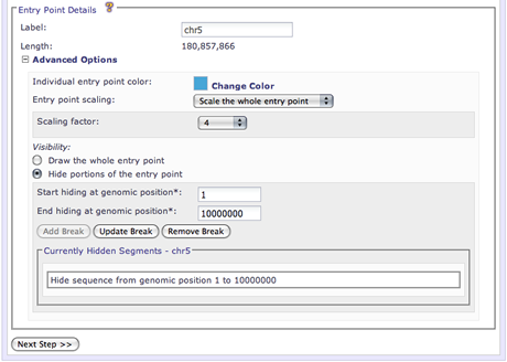
Specify the label for the entry point that will appear if Draw entry point labels: is enabled.
If Color entry points is enabled in the Specification for All Entry Points section, then a user can specify separate colors for each entry point. This option is in the Advanced Options.
Specify a global scale for the entire entry point or a local scale for portions of an entry point. The Entry Point Scales section describes this option in more detail.
Specify portions of the entry point to hide. The Entry Point Breaks section describes this option in more detail.
View the axis scaling tutorial from Circos →
The Entry point scaling section allows a user to specify regions of the image that should be zoomed in or out. Axis scaling is a powerful feature of Circos that gives the user power to focus a viewers attention on areas of the image that are deemed important. With scaling, you can zoom in on areas of the image that are dense with data or zoom out regions that are barren. There are two modes of axis scaling available:
-
Global scaling
Global scaling can be selected by choosing the Scale the whole entry point option from the interface. In this mode, the user specifies the scaling factor that will affect the entire selected entry point. Values greater than zero will effectively zoom in on that entry point. Values less than zero will zoom the selected entry point out.
-
Local scaling
Local scaling can be selected by choosing the Scale parts of the entry point option from the interface. In this mode, the user can localize the scale to only desired sections of the selected entry point. A user is required to specify the starting and ending genomic positions of the region to scale. Values greater than zero will effectively zoom in on that entry point. Values less than zero will zoom the selected entry point out.
View the axis breaks tutorial from Circos →
The Visibility section of the interface allows a user to add axis breaks to the entry point. By adding an axis break, a user can effectively hide sections of the entry point so they are not drawn. Axis breaks can be used to hide uninteresting areas of an entry point from view. A user is required to specify the staring and ending genomic positions for the axis break (the start and end positions of the entry point to hide).
In the Ideogram Specification section on the Specify Ideogram Details tab, a user can control some properties that affect the overall drawing of the circular image. The available options are describe below.
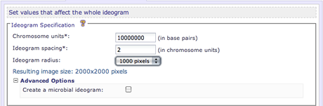
The chromsome units parameter defines a multiplier which can be applied to many other variable values within the configuration files. It is highly recommended to leave the value of the chromosome units as-is. However if you notice spacing issues in your image, this value can be adjusted to try to resolve those problems. This option is required.
Control the amount of whitespace between each entry point ideogram in the image. This value is required and should be specified in relation to the specified value of chromosome units. For example, if a user would like the equivalent spacing of 20 megabases between each ideogram and the chromosome units option is set to 10,000,000 (10 Mb), then a value of 2 would accomplish this. This option is required.
Specify the radius of the circular image. The radius value controls the resulting image size. This value can must be an integer greater than zero. Larger radius sizes create larger and higher resolution images, smaller radius sizes create smaller and lower resolution images.
This option can be used to create the equivalent image of a microbial genome. By selecting this option, Circos will create a closed circle image resembling a traditional microbial genome image. This option is in the Advanced Options.
View the tick marks tutorial from Circos →
Tick marks can provide visual cues to viewers so they can easily understand the scale and positioning of the data in your images. Tick marks can be added to the ideogram through the Tick Mark Settings section on the Specify Ideogram Details tab.
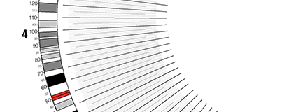
A tick mark is represented in the image as a line radiating outwards from the ideograms, spaced evenly at designated intervals. Each tick mark can also be accompanied by a tick mark label that informs viewers the spacial position of each tick. A user is required to specify the spacing of each tick mark but can also control the size of the mark and the size of the tick label. The available user options are described below.
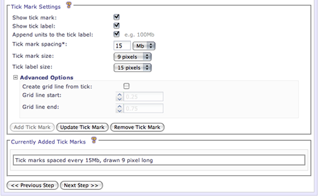
Enable/disable the selected tick mark for drawing. This is useful to temporarily turn off a tick mark without having to delete it.
Enable/disable the selected tick mark label for drawing. This is useful to temporarily turn off a tick mark without having to delete it.
The specified magnitude of each tick mark can be appended to the tick mark label to help a viewer better understan the genomic position of the tick mark and annotation in the image.
The interval to space each tick mark. This option is required.
The length (in pixels) of each tick mark that will be drawn.
The font size for the accompanying tick label, if drawn.
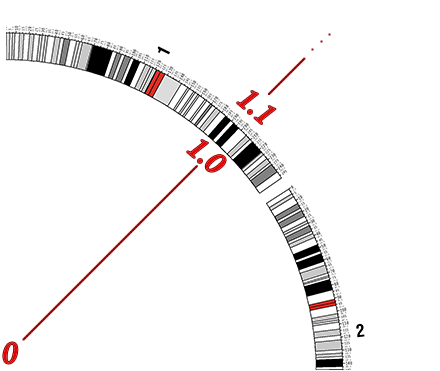
Every tick mark can be specified to add a complimentary grid line. These grid lines radiate from the specified start and end positions. Grid lines can be useful for relating genomic position inside of the ideogram where annotation data will be drawn. Grid lines will be drawn on top of any highlights in the image but will be drawn underneath all other data. This option is in the Advanced Options.
An example of grid lines created from tick marks:
The radial start position for the grid line created from this tick mark. Radial positions must be greater than zero. This option is in the Advanced Options.
The radial end position for the grid line created from this tick mark. Radial positions must be greater than zero. This option is in the Advanced Options.
To add a tick mark, specify values for the desired options and click the Add Tick Mark button. The tick mark will be added for drawing in the ideogram.
To update the options for a tick mark, select the tick mark from the Currently Added Tick Marks List. The values for the selected tick mark will appear in the corresponding widgets. Make the desired changes and then click the Update Tick Mark button. If the button is not clicked then the changes will be lost.
To remove a tick mark from the image, select the tick mark from the Currently Added Tick Marks List. Click the Remove Tick Mark button to completely remove the tick mark.
Any annotation track that exists in your Genboree database can be added to your Circos image and visualized in a variety of drawing types. These data plots are drawn radially outward from the center of the circle and will be drawn in the correct genomic positions. The circular composition of the data makes it extremely useful for visualizing intra- and inter-chromosomal relationships.
View the 2D plots tutorial from Circos →
Circos supports a variety of 2D plot types that can be used to draw annotation data. In this interface, a subset of those types are supported: highlight, scatter plot, line plot, histogram, tiles, heatmaps and links. These track types are described below along with the available options.
It is important to discuss a critical option that pertains to all plot types, links and highlights. All tracks need to specify the starting and ending radial positions for where within the circular image they should be drawn. A radial position is a decimal value that is greater than zero. A radial position value between 0 - 1 will be drawn inside the circle. A radial value greater than 1 will be drawn outside the circle. Drawing annotation on both sides of the circular ideogram can produce more informative images as well as provide more drawing space to reduce clutter. Creative uses of these values can also create some visually attractive images. When adding annotation tracks, consider the value of the radial options carefully as they control the overall layout of your data.
-
Highlight - Annotations are represented as a colored highlight, either inside the circular
image or the highlight can be drawn on top of the ideogram itself.
View the highlight tutorial from Circos →
-
Inner radius
The inner radius is the starting position for this plot. The value must be greater than zero and is typically less than the specified outer radius. Press the up and down arrows to increment and decrement the radius values. Holding down the shift key while pressing the up and down arrow will change the value by 0.1. This option is required.
-
Outer radius
The outer radius is the ending position for this plot. The value must be greater than zero and is typically greater than the specified inner radius. Press the up and down arrows to increment and decrement the radius values. Holding down the shift key while pressing the up and down arrow will change the value by 0.1. This option is required.
-
Draw the highlight on the ideogram
This option controls whether the ideogram should be drawn inside the circle or on top of the entry point ideograms themselves. Enabling this option will make Circos ignore the inner and outer radius values. This is called an ideogram highlight.
-
Highlight fill color
The desired color to fill the highlight with.
-
Highlight stroke color
The desired color to stroke the highlight with. A stroke will be drawn as a one pixel border around the highlight in the specified color. This option is in the Advanced Options.
-
Inner radius
-
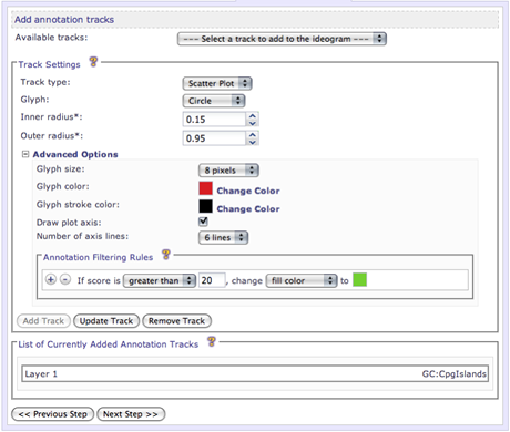
Scatter plot - Annotations are represented as a colored glyphs at their corresponding genomic position.
View the scatter plot tutorial from Circos →
-
Glyph
The type of marker to be used for each piece of annotation. Options are: circle, rectangle and triangle.
-
Inner radius
The starting position for this plot. See highlight for more information.
-
Outer radius
The ending position for this plot. See highlight for more information.
-
Glyph size
The size, in pixels, to draw each glyph representing a piece of annotation. This option is in the Advanced Options.
-
Glyph color
The fill color for all glyphs. This option is in the Advanced Options.
-
Glyph stroke color
The stroke color for all glyphs. The stroke will be drawn as a one pixel border around each glyph in the specified color. This option is in the Advanced Options.
-
Draw plot axis
Enable/disable the drawing of a scale axis for the plot. Axis lines will be drawn at set intervals from the start of the plot to the end of the plot. They will be drawn as 2 pixel lines in a light gray color. An axis is useful to help give viewers a sense of relative scale of the annotation values in the plots. This option is in the Advanced Options.
-
Number of axis lines
The number of axis lines to be drawn if the axis is enabled. This option is in the Advanced Options.
-
Glyph
-
Line plot - Similiar to the scatter plot but instead of each annotation being represented as
a glyph, they are connected with a line.
View the line plot tutorial from Circos →
-
Inner radius
The starting position for this plot. See highlight for more information.
-
Outer radius
The ending position for this plot. See highlight for more information.
-
Line color
The color the connecting line will be drawn in.
-
Line thickness
The thickness of the connecting line. This option is in the Advanced Options.
-
Draw plot axis
Enable/disable the drawing of a scale axis for the plot. See the scatter plot description for more information. This option is in the Advanced Options.
-
Number of axis lines
The number of axis lines to be drawn if the axis is enabled. This option is in the Advanced Options.
-
Inner radius
-
Histogram - Circos' histograms are a slight variation on the line plot. In a line plot, adjacent
points are connected by a straight line whereas in a histogram the points form a step-like trace.
View the histogram tutorial from Circos →
-
Inner radius
The starting position for this plot. See highlight for more information.
-
Outer radius
The ending position for this plot. See highlight for more information.
-
Histogram line color
The color the histogram line will be drawn in.
-
Fill histogram area
Enable/disable filling the area under the histogram with a specified color. This option is in the Advanced Options.
-
Histogram area fill color
The fill color for the area under the histogram, if fill is enabled. This option is in the Advanced Options.
-
Histogram orientation
Orientation for the histogram to be drawn. Setting orientation to out will draw smaller values closer to the center of the circle than larger ones. This option is in the Advanced Options.
-
Inner radius
-
Tiles - Annotations are represented as a colored rectangles that span their corresponding genomic position.
Tiles will stack within their designated track to avoid overlap.
View the tiles tutorial from Circos →
-
Inner radius
The starting position for this plot. See highlight for more information.
-
Outer radius
The ending position for this plot. See highlight for more information.
-
Tile color
The color that all the tiles should be filled with.
-
Tile orientation
The direction to start drawing the tiles from. When Out is specified, tiles will stack from the inner radius out towards the outer radius. When In is specified, tiles will stack from the outer radius in towars the inner radius.
-
Number of tile layers to draw
Number of allowed tile layers. The tile data plot will attempt to draw tiles so that they do not overlap. When an overlap is detected, the overlapping tile will be drawn in a new layer. The extent to which this occurs is limited by the number of tile layers specified. If the layer limit has been reached, tiles will begin to overlap, either by collapsing or being hidden. The Circos tutorial image explains the stacking process of times in more depth.
-
Stroke color
The color that all the tiles will be stroked with. The stroke is a single pixel border. This option is in the Advanced Options.
-
Tile thickness
The thickness, in pixels, of each rectangular tile. This option is in the Advanced Options.
-
Display for overflow tiles
The mode of operation for tiles that cannot be drawn in a layer and thus overflow onto other tiles. If Collapse is specified then overlapping tiles will collapse onto other tiles and be colored different. If Hide is specified, then tiles that overlap will not be drawn in the image. This option is in the Advanced Options.
-
Overflow tiles color
The fill color for any overlapping tiles that are specified to be drawn in collapsed mode. This option is in the Advanced Options.
-
Draw plot axis
Enable/disable the drawing of a scale axis for the plot. See the scatter plot description for more information. This option is in the Advanced Options.
-
Number of axis lines
The number of axis lines to be drawn if the axis is enabled. This option is in the Advanced Options.
-
Inner radius
-
Heatmap - Annotations are represented as a colored rectangles whose drawing color is determined as a function of their
annotation value. Heatmaps combine the utility of highlights and data plots.
View the heatmap tutorial from Circos →
-
Inner radius
The starting position for this plot. See highlight for more information.
-
Outer radius
The ending position for this plot. See highlight for more information.
-
Heatmap colors
The list of heatmap colors. At least one color is required. The drawing color of the annotations is determined by the following function: color_index = num_colors * (anno. value-min)/(max-min)
-
Draw plot axis
Enable/disable the drawing of a scale axis for the plot. See the scatter plot description for more information. This option is in the Advanced Options.
-
Number of axis lines
The number of axis lines to be drawn if the axis is enabled. This option is in the Advanced Options.
-
Inner radius
-
Links - Genomic positions can be linked if a user-specified attribute value is equivalent at differing positions.
Links are visually represented as arching lines who terminal points are the linked genomic positions.
View the link tutorial from Circos →
-
Link this track to
The other annotation track to link the selected one to. A track can be linked to itself. When a track is linked to another, genomic positions that share a common value in the desired attribute will be linked with a line.
-
Link tracks when values are equal in
The attribute to examine and determine if positions are linked. When the values of this selected attribute are equal, a link will be created between the genomic positions where that annotation exists.
-
Start & end radius
The radial position that the line representing the link will be drawn from. This option is similiar to the inner and outer radius options of the 2D plots.
-
Maximum number of links to draw
The number of links to be displayed in the final image. If the image appears too cluttered because a high volume of links are visible, consider setting the value for this option lower.
-
Link color
The drawing color for the links. Links are drawn as 2 pixel colored lines.
-
Draw links as ribbons
Draw the links as ribbons rather than 2 pixel lines. A normal link has a set thickness and did not convey the span of genomic positions the link covered. By drawing links as ribbons, a viewer can observe the sizes of the linked regions. This option is in the Advanced Options.
-
Bezier radius for links
The radius of the bezier control point. Increasing this value makes the line curve more. This option is in the Advanced Options.
-
Link this track to
To add an annotation track to the image, first select the track to add from the Available tracks list. Select the 2D plot type for the track and specify the desired options and rules. Click the Add Track button to add the annotation track. By default, the track will be drawn at the highest layer, on top of all other annotation tracks in the image, if any overlap exists.
To update a track, select it from the List of Currenly Added Annotation Tracks. Selecting the track item will populate the UI widgets Track Settings section with the currently set track options. Change the desired options and click the the Update Track to save the changes. If the button is not clicked then the changes will be lost.
The layering of an annotation track can be changed by selecting the track item from the list and dragging the item up or down to the desired position. Moving a track to a higher numbered layer (dragging down) will cause the track to be drawn on top of lower numbered tracks. The new layer position will automatically be saved on release.
To remove a track, select it from the List of Currently Added Annotation Tracks. Click the Remove Track button to completely remove the track.
All 2D data plots, except the histogram type, support annotation filtering rules. Here are user can add rules to filter the annotation data so that the resulting image will be affected. A condition is required, based on the annotation score, and if the condition is met, the rule will be enforced. The available properties that the rule can alter are dependent upon the type of plot selected. Rules can be useful to distinguish annotations that have differring values.
When you have finished specifying how your Circos image should be created, you can submit the job to the Genboree servers for processing by going to the Submit tab.
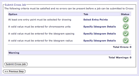
The Submit tab also informs you of the status of you current Circos configuration. To submit a job, there must be no errors in your configuration and all of the required options must be specified. The options table at the top of the page will display the options and their current status.
The errors table will inform you of any specified options that have invalid values set. All errors must be fixed to submit a job.
The warnings table will provide information about specified options that have values that might produce unexpected results. The warnings do not have to be removed before submitting a Circos job and can be ignore if they are expected.
Upon submitting the job for processing, the server will be sent your request and return an acknowledgment. If an error occurs while communicating with the server, an error message will be returned. If the request occurs successfully, you will be informed and given a Job ID for your Circos job. When the job has finished processing, you will be notified via email and provided a link to visit so you can view the results.
If you have any questions about a submitted Circos job, contact your Genboree administrator and provide them with your Circos Job ID so they can properly assist you.

|
© 2001-2026 Baylor College of Medicine
Bioinformatics Research Laboratory (400D Jewish Wing, MS:BCM225, 1 Baylor Plaza, Houston, TX 77030) |